6.5 Z Scores
We have looked at the mean as a model; and we have learned some ways to quantify total error around the mean, as well as some good reasons for doing so. But there is another reason to look at both mean and error together. Sometimes, by putting the two ideas together it can give us a better way of understanding where a particular score falls in a distribution.
A student (let’s call her Zelda) has a thumb length of 65.1 mm. What does this mean? Is that a particularly long thumb? How can we know? By now you may be getting the idea that just knowing the length of one thumb doesn’t tell you very much.
To interpret the meaning of a single score, it helps to know something about the distribution the score came from. Specifically, we need to know something about its shape, center and spread.
We know that this student’s thumb is about 5 mm longer than the average. But because we have no idea about the spread of the distribution, we still don’t have a very clear idea of how to judge 65.1 mm thumb length. Is a 5 mm distance still pretty close to the mean, or is it far away? It’s hard to tell without knowing what the range of thumb lengths looks like.
Although SS will be really useful later, for this purpose it stinks. 65.1 and 11,880 don’t seem like they belong in the same universe! Variance will also be useful, but its units are still somewhat hard to interpret. It’s hard to use squared millimeters as a unit when trying to make sense of unsquared millimeters.
Standard deviation, on the other hand, is really useful. We know that Zelda’s thumb is about 5 mm longer than the average thumb. But now we also know that, on average, thumbs are 8.7 mm away from the mean, both above and below. Although Zelda’s thumb is above average in length, it is definitely not one of the longest thumbs in the distribution. Check out the histogram below to see if this interpretation is supported.
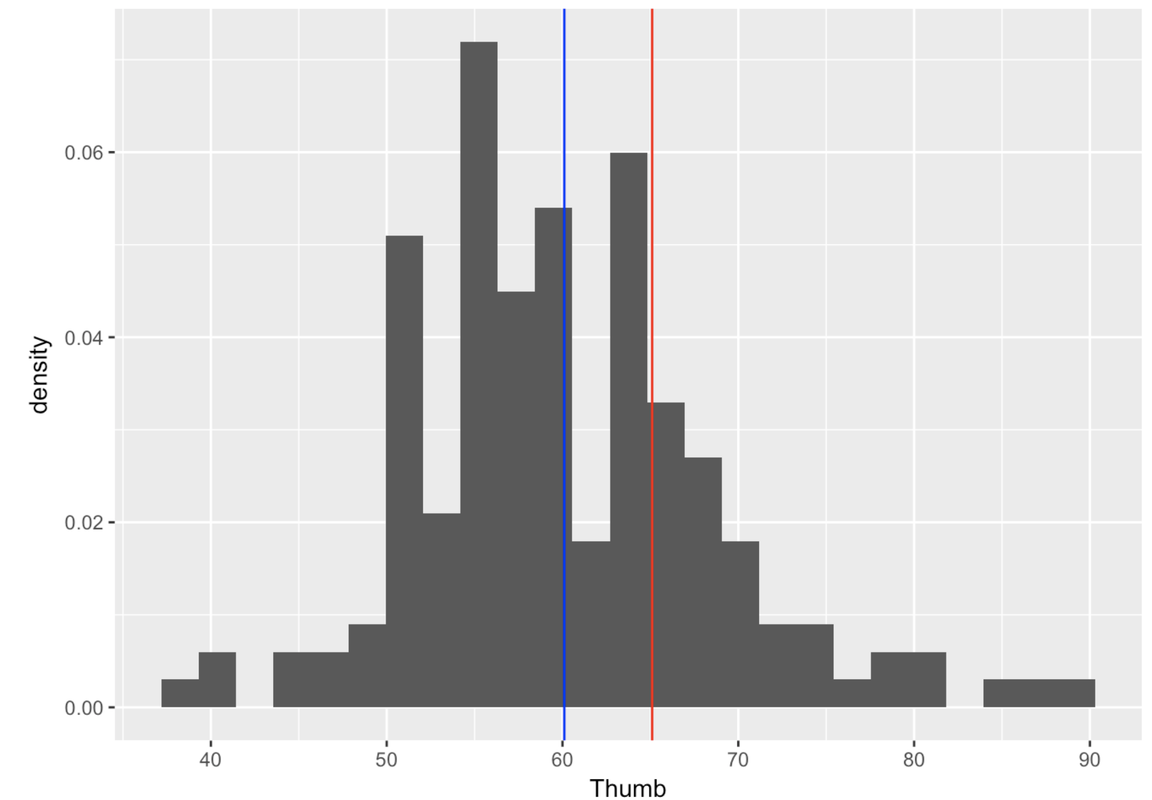
The mean of thumb length is shown in blue, and Zelda’s 65.1 mm thumb is shown in red.
Combining Mean and Standard Deviation
In the Thumb situation, we find it valuable to coordinate both mean and standard deviation in order to interpret the meaning of an individual score. Now, let’s introduce a measure that will combine these two pieces of information into a single score: the z score.
Let’s say you know that the mean score across all players of the game is 35,000. How would that help you? Clearly it would help. You would know that the score of 37,000 is above the average by 2,000 points. But even though it helps you interpret the meaning of the 37,000, it’s not enough. What it doesn’t tell you is how far above the average 37,000 points is in relation to the whole distribution.
Let’s say the distribution of scores on Kargle is represented by one of these histograms. Both distributions have an average score of 35,000. But in the distribution on the top (#1), the standard deviation is 1,000 points, while on the bottom (#2) the standard deviation is 5,000 points. The blue line depicts the mean, and the red line depicts our friend’s score of 37,000.
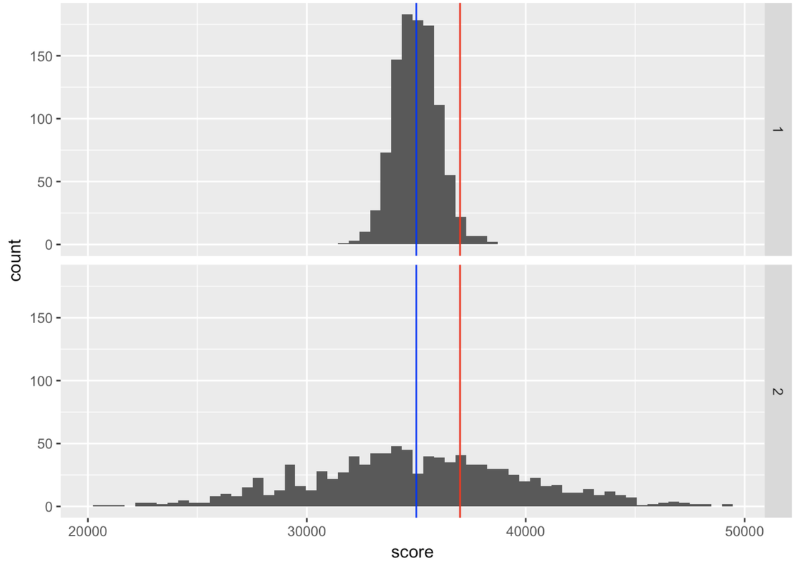
Clearly your friend would be an outstanding player if Distribution 1 were true. But if Distribution 2 were true, they would be just slightly above average.
We can see this visually just by looking at the two histograms. But is there a way to quantify this intuition? One way to do this is by transforming the score we are trying to interpret into a z score using this formula:
\[z_{i}=\frac{Y_{i}-\bar{Y}}{s}\]
Let’s apply this formula to our video game score of 37,000 based on each of the two hypothetical distributions (#1 and #2) above.
We show you the R code for calculating the z score for a score of 37,000 if Distribution 1 is true. Write similar code to calculate z score if Distribution 2 is true.
require(coursekata)
# z-score if distribution 1 were true
(37000 - 35000)/1000

# z-score if distribution 2 were true
(37000 - 35000)/1000
(37000 - 35000)/5000
ex() %>% {
    check_output_expr(., "(37000 - 35000)/1000")
    check_output_expr(., "(37000 - 35000)/5000", missing_msg="Did you divide by the sd of the second distribution?")
}[1] 2[1] 0.4In both cases, the numerator is the same: 37,000 (the individual score) minus the mean of the distribution, which equals 2,000. The denominators for the two z scores are different, though, because the distributions have different standard deviations. In distribution #1, the standard deviation is 1,000. So, the z score is 2,000 divided by 1,000, or 2. For the other distribution, the standard deviation is 5,000. So, the z score is 2,000 divided by 5,000, or .40.
If we did this calculation without parentheses, the calculation would be 37,000 - (35,000 / 5,000) because order of operations, our cultural conventions for how we do arithmetic, says that division is done before subtraction.
A z score represents the number of standard deviations a score is above (if positive) or below (if negative) the mean. So, the units are standard deviations. A z score of 2 is two standard deviations above the mean. A z score of 0.4 is 0.4 standard deviations above the mean.
A z score of 2 is more impressive—it’s two standard deviations above the mean. It should be harder to score two standard deviations above the mean than to score 0.4 (or less than one half) a standard deviation above the mean.
Standard deviation (SD) is roughly the average deviation of all scores from the mean. It can be seen as an indicator of the spread of the distribution. A z score uses SD as a sort of ruler for measuring how far an individual score is above or below the mean.
A z score tells you how many standard deviations a score is from the mean of its distribution, but doesn’t tell you what the standard deviation is (or what the mean is). Another way to think about it is that a z score is a way of comparing a deviation of a score (the numerator) to the standard deviation of the distribution (the denominator).
Let’s use z scores to help us make sense of our Thumb data. Calculate the z score for a 65.1 mm thumb.
require(coursekata)
# Thumb_stats will have mean and sd in it
Thumb_stats <- favstats(~ Thumb, data = Fingers)

# write code to calculate the z score for a 65.1 mm Thumb
Thumb_stats <- favstats(~Thumb, data = Fingers)
(65.1 - Thumb_stats$mean) / Thumb_stats$sd
ex() %>% {
    check_object(., "Thumb_stats") %>% check_equal()
    check_output_expr(., "(65.1 - Thumb_stats$mean) / Thumb_stats$sd")
}[1] 0.5725349A single z score tells us how many standard deviations away this particular 65.1 mm thumb is from the mean. Because the standard deviation is roughly the average distance of all scores from the mean, it is likely that most scores are clustered between one standard deviation above and one standard deviation below the mean. It is less likely to find scores that are two or three standard deviations away from the mean. Z scores give us a way to characterize scores in a bit finer way than just bigger or smaller than the mean.
Using Z Scores to Compare Scores From Different Distributions
One more use for the z score is to compare scores that come from different distributions, even if the variables are measured on different scales.
Here’s the distribution of scores for all players of the video game Kargle again. We know that the distribution is roughly normal, the mean score is 35,000, and the standard deviation is 5,000.
Her z score is +2. Wow, two standard deviations from the mean! Not a lot of scores are way up there.
Now let’s say you have another friend who doesn’t play Kargle at all. She plays a similar game, though—Spargle! Spargle may be similar, but it has a completely different scoring system. Although the scores on Spargle are roughly normally distributed, their mean is 50, and the standard deviation is 5. This other friend has a high score of 65 on Spargle.
Now: what if we want to know which friend, in general, is a better gamer? The one who plays Kargle, or the one who plays Spargle? This is a hard question, and there are lots of ways to answer it. The z score provides one way.
We’ve summarized the z scores for your two friends in the table below.
| Player | Player Score | Game Mean | Game SD | Player Z Score |
| Kargle Player | 45,000 | 35,000 | 5,000 | +2.0 |
| Spargle Player | 65 | 50 | 5 | +3.0 |
Looking at the z scores helps us to compare the abilities of these two players, even though they play games with different scoring systems. Based on the z scores, we could say that the Spargle player is a better gamer, because she scored three standard deviations above the mean, compared with only two standard deviations above the mean for the Kargle player.
Of course, nothing is really definite with such comparisons. Someone might argue that Spargle is a much easier game, and so the people who play it tend to be novices. Maybe the Kargle player is better, because even though her z score is lower, she is being compared to a more awesome group of gamers!