9.5 A Mathematical Model of the Sampling Distribution of b1
The early statisticians who developed the ideas behind sampling distributions and p-values didn’t have computers. They could only imagine what it might be like to shuffle() their data to imitate a random DGP. What we have been able to do with R would seem like a miracle to them! Instead of using computational techniques to create sampling distributions, the early statisticians had to develop mathematical models of what the sampling distributions should look like, and then calculate probabilities based on these mathematical distributions.
In fact, the p-value you see in the ANOVA table generated by the supernova() function (as well as most other statistical software) is calculated from a mathematical model of the sampling distribution.
The code in the window below fits the Condition model to the TipExperiment data and saves the model as Condition_model. Use supernova() to generate the ANOVA table for this model, and look at the p-value (in the right-most column of the table).
require(coursekata)
# This code finds the best fitting Condition model
            Condition_model <- lm(Tip ~ Condition, data = TipExperiment)

            # Generate the ANOVA table for this model
# This code finds the best fitting Condition model
Condition_model <- lm(Tip ~ Condition, data = TipExperiment)

# Generate the ANOVA table for this model
supernova(Condition_model)
ex() %>%
    check_function("supernova") %>%
    check_result() %>%
check_equal()Analysis of Variance Table (Type III SS)
Model: Tip ~ Condition
SS df MS F PRE p
----- --------------- | -------- -- ------- ----- ------ -----
Model (error reduced) | 402.023 1 402.023 3.305 0.0729 .0762
Error (from model) | 5108.955 42 121.642
----- --------------- | -------- -- ------- ----- ------ -----
Total (empty model) | 5510.977 43 128.162 The p-value from supernova(), rounded to the nearest hundredth, is about .08, which is very close to what we calculated using our sampling distribution of 1000 shuffled \(b_1s\). The approach that uses the mathematical model is not necessarily better than the shuffling approach; the point is that both methods yield a similar result. (Although running supernova() is faster, some people find the concept of sampling distribution easier to understand when they generate the sampling distribution of \(b_1\)s using shuffle().)
The t-Distribution
The mathematical function that supernova() uses to model the sampling distribution of \(b_1\) (as well as the sampling distributions of many other parameter estimates) is known as the t-distribution. The t-distribution is closely related to the normal distribution, and in fact it looks very much like the normal distribution.
In the figure below we have overlaid the t-distribution (depicted as a red line) on top of the sampling distribution we constructed using shuffle(). You can see that it looks very much like the normal distribution you learned about previously.
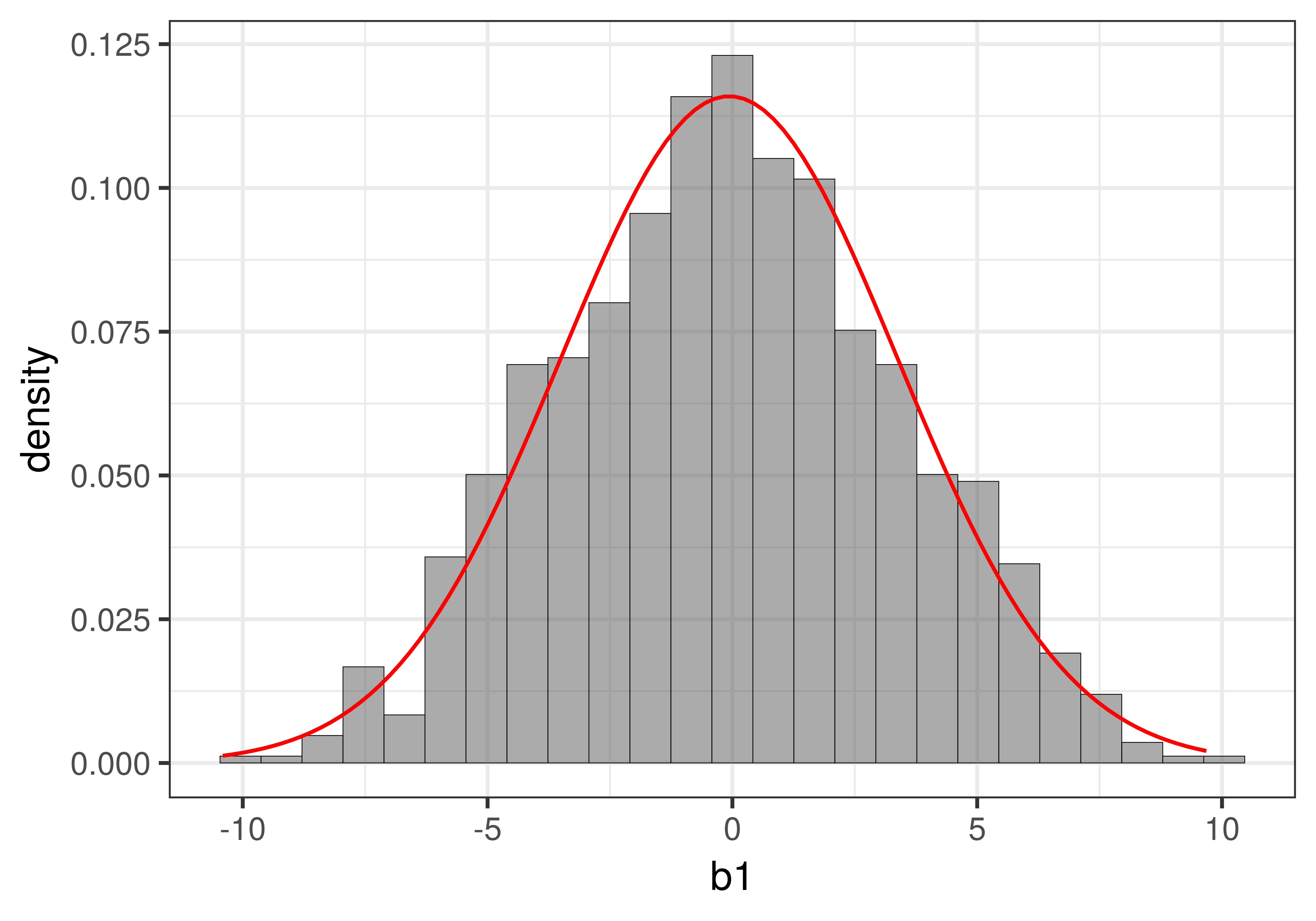
Whereas the sampling distribution we created using the shuffle() function looks jagged (because it was made up of just 1000 separate \(b_1\)s), the t-distribution is a smooth continuous mathematical function. If you want to see the fancy equation that describes this shape, you can see it here.
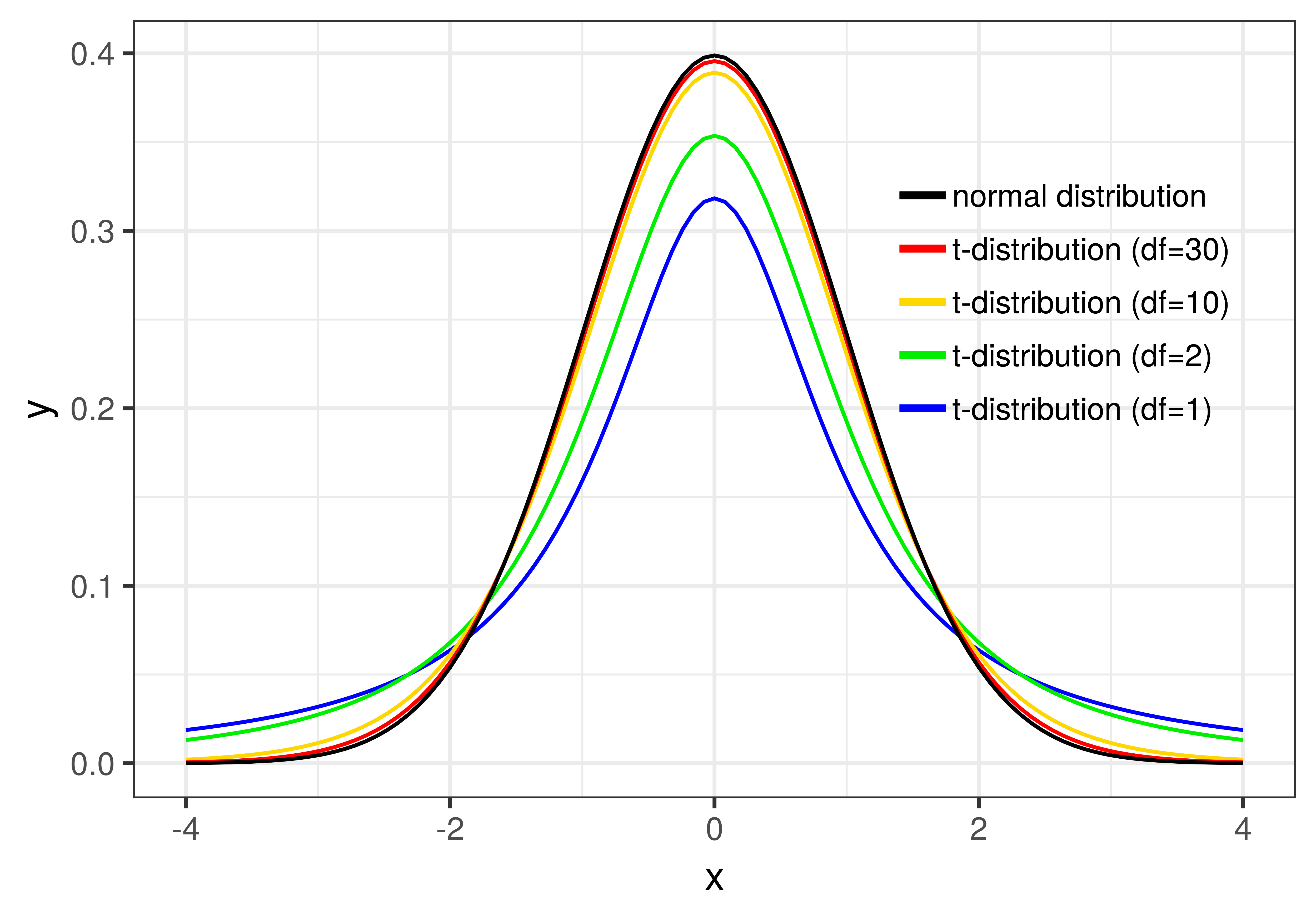
Whereas the shape of the normal distribution is completely determined by its mean and standard deviation, the t-distribution changes shape slightly depending on how many data points are included in the samples that make up the sampling distribution. (Actually, \(t\) is based on degrees of freedom, or \(d\!f\), within each group, which you’ve learned is \(n-1\). For the tipping study, the \(d\!f\) is 42, 21 for each group).
You can see how \(d\!f\) affects the shape of the t-distribution in the figure below. Once the degrees of freedom reaches 30, however, the t-distribution looks very similar to the normal distribution.
Using the t-Distribution to Calculate Probabilities
In the sampling distribution you created using shuffle() you were able to just count the number of \(b_1\)s more extreme than the sample \(b_1\) in order to calculate the p-value. The t-distribution works the same way, except that it takes some complicated math to calculate the probabilities in the upper and lower tails. Fortunately, you don’t have to do this math; R will do it for you (e.g., when you tell it to use the supernova() function).
The Two-Sample T-Test
If you’ve taken statistics before you probably learned about the t-test. The t-test is used to calculate the p-value for the difference between two independent groups. The tipping experiment is just such a case: the \(b_1\) we’ve been working with is the difference between two groups of tables, those that got the smiley face and those that did not.
You can use R to do a t-test on the tipping data:
t.test(Tip ~ Condition, data = TipExperiment, var.equal=TRUE)If you run this code it will give you the p-value of .0762, which is exactly what you saw in the ANOVA table produced by supernova(). Even though the supernova() output does not show you the t-statistic or other details of how it calculates the p-value, behind the scenes it uses the t-distribution for calculating p-values.
Although we want you to know what a t-test is, we don’t recommend using it. The technique you have learned, of creating a two-group model and comparing it with the empty model, is far more powerful and generalizable than the t-test. But if someone asks if you learned the t-test, you can say yes. (The test you did using shuffle() is sometimes called a randomization test or permutation test.)