5.2 Modeling a Distribution with a Single Number
Building on this concept of model, let’s now develop what we mean by a statistical model. Whereas in the previous section we were building a model to help us estimate the area of the state of California, we now want to build a model we can use to characterize a distribution.
As you will see in subsequent chapters, statistical models are very useful. We use them to summarize distributions. We use them to make predictions about what the next observation added to a sample distribution might be. And we use them to explain variation in one variable with another. But we will start with the simplest model, which uses a single number to characterize a distribution.
At its most basic level, a statistical model can be thought of as a function that produces a predicted score for each observation in a distribution. By “function” we don’t mean an R function; we mean a mathematical procedure for generating a number based on the data. The simplest models we consider generate the same predicted score for every observation in a distribution—a single number to characterize a whole distribution.
If you had to pick one number to represent an entire distribution, how would you pick it? And what would it be? Thought of in a different way: if you wanted to predict what the value of the next randomly chosen observation would be, what would be your best prediction?
Depending on how a variable is measured (e.g., quantitative or categorical), and on the shape of the distribution, we will use different procedures (or different functions) for choosing one number as a model.
For a quantitative variable whose distribution is roughly symmetrical and bell shaped, a number right in the middle might be the best-fitting model. (Remember, we aren’t saying that such a simple model is a good model—just better than nothing!) If a distribution is skewed left or right, the best model might be a number toward where the middle would be if you ignored the long tail on one side or the other. For a categorical variable, the best model is generally the category that is most frequent.
Model and Error
Let’s zero in on just distributions of quantitative variables. Take a look at the two distributions below for variables 1 and 2.
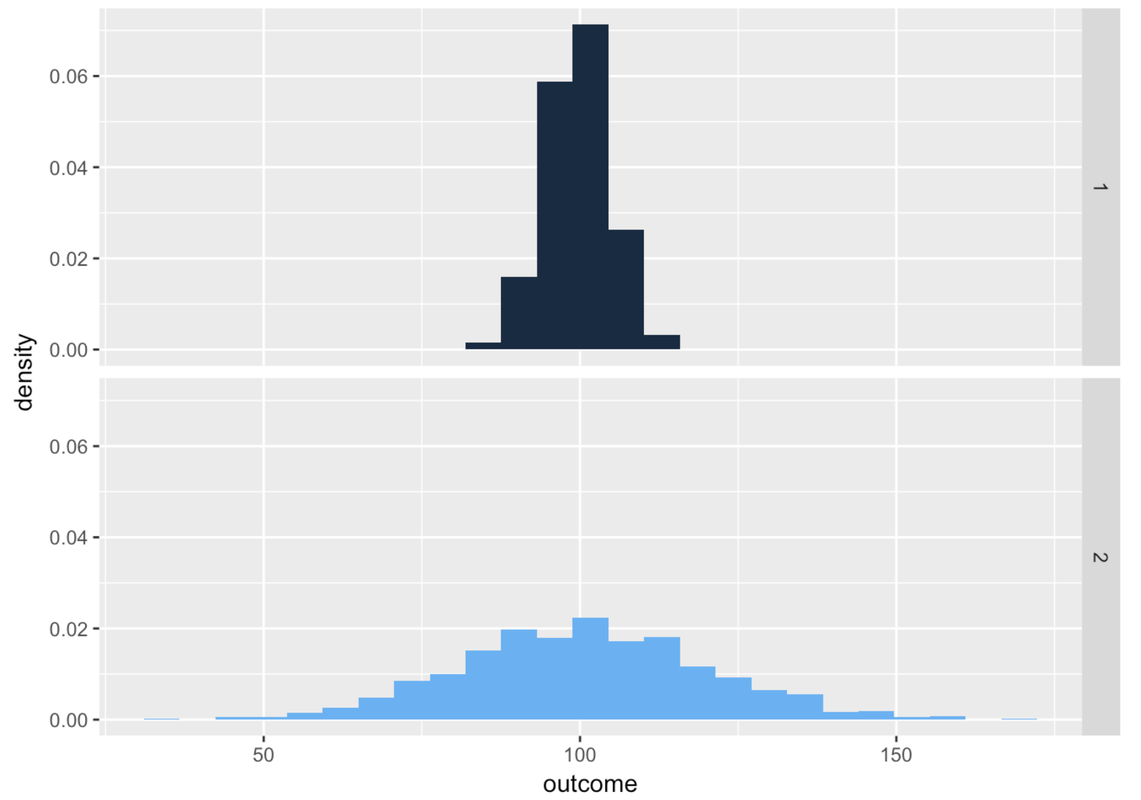
A single number—even a well-chosen number—is not a very good model. It may be a better model for variable 1 than variable 2 above, but it’s still not very good. Most scores are not the same as the number we choose as the model.
Which brings us to another important concept: once we choose a number to model a distribution (and we’ll talk soon about how we do that), we can think of the variation around that number as error, just as we considered the parts of California not covered by geometric shapes as error.
If we use a single number to model the distribution of a quantitative variable, error from the model can be seen as deviations of the observed scores from that predicted number. As we just saw, a one-number model for a distribution with less spread seems to have less error, and thus a better fit, than a one-number model for a distribution with more spread. The reason for this is that the error around the model is greater for the distribution with more spread.
The idea of modeling a distribution with a single number gives us a more concrete and detailed way of thinking about our models. Whereas we thought about the California example like this:
AREA OF CALIFORNIA = AREA OF GEOMETRIC FIGURES + ERROR
We can think of a statistical model like this:
DATA = MODEL + ERROR
Each data point in a distribution can be decomposed into two parts: the model (i.e., the number we are using to represent the whole distribution), and the data point’s deviation from the model (the error).