11.3 Shuffle, Resample, and Standard Error
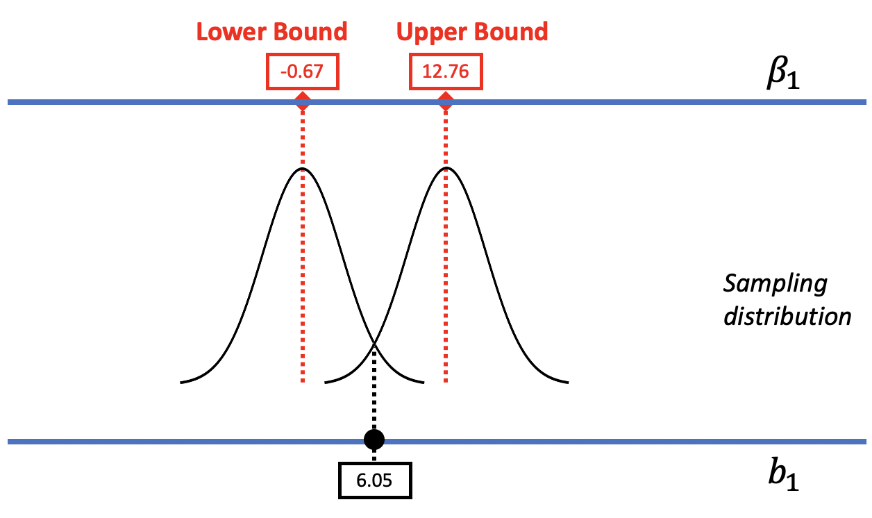
We started with the idea that we could slide the sampling distribution of \(b_1\) up and down to find the lower and upper bounds of the confidence interval. Noticing that the center of this confidence interval was right at the sample \(b_1\), we used resample() to bootstrap a sampling distribution that would be centered at the sample \(b_1\). This helped us calculate the upper and lower bounds.
To do all this, however, we assumed that the sampling distributions generated from different DGPs (e.g., different values of \(\beta_1\) such as $0, $6.05, $13, etc.) would all have the same shape and spread. We have now used two methods to create sampling distributions of \(b_1\), each based on a different DGP. Do these sampling distributions have the same shape and spread?
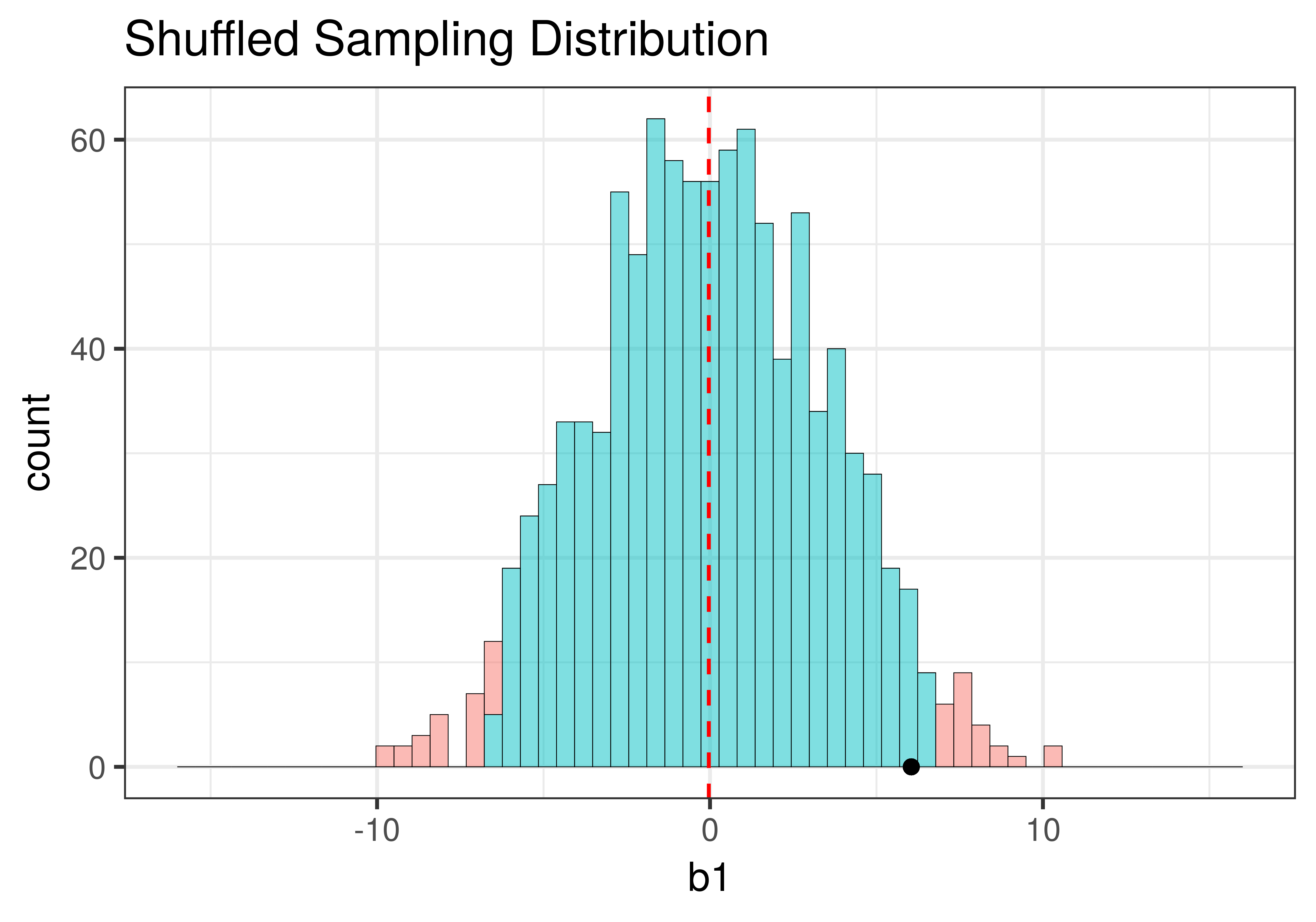
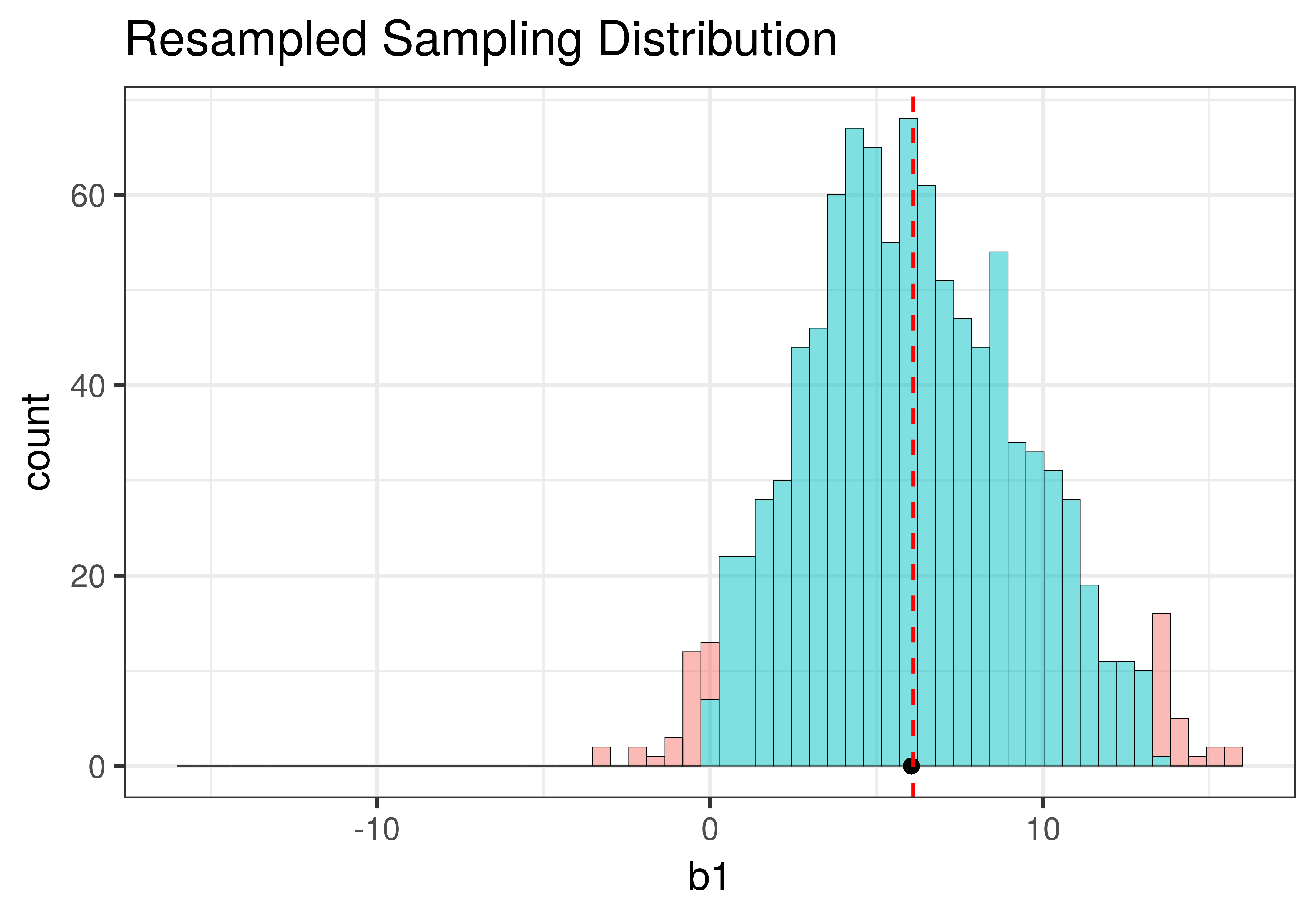
Using shuffle(), we simulated a DGP in which the \(\beta_1=0\) (that is, the empty model is true). It’s depicted in the left panel of the figure below. Using resample() (right panel of the figure), we simulated a DGP in which the true value of \(\beta_1=6.05\), the same as the sample \(b_1\).
|
|
Although the centers of the two sampling distributions are different, the shapes of the two distributions are similar. Both are roughly normal and symmetrical. Though the one produced by resample() appears to be somewhat asymmetrical – it’s skewed a little to the right – we will, for now, consider it close enough to symmetrical.
The Importance of Standard Error
The most important feature of the sampling distributions, however, is their width. We can eyeball the range from the histograms above (e.g., both are around 20) and already see that they are similar. A more commonly used measure of spread is standard error. In the code window below, use favstats() to calculate the standard errors of the two sampling distributions: made from shuffle and resample. (We have included code to create the two sampling distributions for you.)
require(coursekata)
sdob1 <- do(1000) * b1(shuffle(Tip) ~ Condition, data = TipExperiment)
sdob1_boot <- do(1000) * b1(Tip ~ Condition, data = resample(TipExperiment))

# use favstats to find the standard error of these sampling distributions
favstats( )
favstats( )
sdob1 <- do(1000) * b1(shuffle(Tip) ~ Condition, data = TipExperiment)
sdob1_boot <- do(1000) * b1(Tip ~ Condition, data = resample(TipExperiment))

# use favstats to find the standard error of these sampling distributions
favstats(~ b1, data = sdob1)
favstats(~ b1, data = sdob1_boot)
ex() %>% {
       check_function(., "favstats", index = 1) %>%
         check_result() %>%
         check_equal()
       check_function(., "favstats", index = 2) %>%
         check_result() %>%
         check_equal()
}In the first output below we show the favstats for the \(b_1\)s created by shuffle(). In the second, we show the favstats created by resample().
       Min       Q1      median       Q3      max        mean       sd    n missing
 -9.954545     -2.5 -0.04545455      2.5 10.22727 -0.03554545 3.498973 1000       0
min Q1 median Q3 max mean sd n missing
-3.219048 3.772727 5.921166 8.480083 15.96154 6.110566 3.381418 1000 0The favstats reveal that the means of the two sampling distributions are roughly as expected: the shuffled distribution has a mean that is fairly close to $0, and the resampled distribution has a mean close to the sample \(b_1\) of $6.05.
While the means are different ($0 versus $6.05), the standard deviations of the two distributions are quite similar to each other: 3.50 for the shuffled distribution, and 3.38 for the resampled distribution. Because these are standard deviations of sampling distributions we call them standard errors.
The fact that the standard errors are similar is an important feature of sampling distributions. The constancy of standard error, along with the shape, is what allows us to assume that we can slide sampling distributions up and down the x-axis when we are constructing a confidence interval.
The standard error is the most important determiner of the width of the confidence interval: the larger the standard error, the wider the confidence interval will be.
A larger standard error means that the spread of the sampling distribution is larger, which in turn means there is more variability (or uncertainty) in our estimate. If there is more variability in the estimate, we should be less confident that our best estimate is a reflection of the true parameter.
A Mathematical Formula for Standard Error
When R models a sampling distribution as a t-distribution, it makes its own calculation of what the standard error is. It does this based on a formula, developed by mathematicians, which is part of something called the Central Limit Theorem.
The Central Limit Theorem provides a way of finding the standard error of a sampling distribution based on the estimated variance of the outcome variable. For the sampling distribution of \(b_1\), when \(b_1\) is the difference between two groups, the standard error can be estimated with this formula:
\[\sqrt{\frac{s_1^2}{n_1} + \frac{s_2^2}{n_2}}\]
Don’t worry, you won’t need to calculate this yourself. We just want you to know what R is doing when it uses a t-distribution. It doesn’t shuffle or bootstrap a sampling distribution and then calculate the standard deviation of the sampling distribution. It just uses this formula.
We can use the following code (no need to remember it) to fit the Condition model of Tip (you’ve done this many times by now), and then to produce the estimates and standard errors for the \(b_0\) and \(b_1\) parameter estimates.
model <- lm(Tip ~ Condition, data = TipExperiment)
summary(model)$coef
Estimate Std. Error t value Pr(>|t|)
(Intercept) 27.000000 2.351419 11.482428 1.546877e-14
ConditionSmiley Face 6.045455 3.325409 1.817958 7.620787e-02
The \(b_1\) estimate is in the second row of the column that says Estimate. As expected, it is $6.05. The standard error of the estimate (which is another way of saying the standard deviation of the sampling distribution) is 3.33.
We now have three different estimates of the standard error of the sampling distribution of \(b_1\): 3.50, 3.38, and 3.33 (from shuffling, resampling, and the mathematical equation, respectively). The important thing to note is that they are all fairly close to one another.
Using the t-Distribution to Construct a Confidence Interval
Just as we used the t-distribution in Chapter 9 to model the sampling distribution of \(b_1\) for purposes of calculating a p-value (the approach used by supernova()), we can use it here to calculate a 95% confidence interval.
In the figure below, we replaced the resampled sampling distribution of \(b_1\)s with one modeled by the smooth t-distribution with its associated standard error. As before, we can mentally move the t-distribution down and up the scale to find the lower and upper bounds of the confidence interval.
The R function that calculates a confidence interval based on the t-distribution is confint().
Here’s the code you can use to directly calculate a 95% confidence interval that uses the t-distribution as a model of the sampling distribution of \(b_1\):
confint(lm(Tip ~ Condition, data = TipExperiment))The confint() function takes as its argument a model, which results from running the lm() function. In this case we simply wrapped the confint() function around the lm() code. You could accomplish the same goal using two lines of code, the first to create the model, and the second to run confint(). Try it in the code block below.
require(coursekata)
# create the condition model of tip and save it as Condition_model
Condition_model <-
confint(Condition_model)
# create the condition model of tip and save it as Condition_model
Condition_model <- lm(Tip ~ Condition, data = TipExperiment)
confint(Condition_model)
ex() %>%
    check_function("lm") %>%
    check_result() %>%
check_equal() 2.5 % 97.5 %
(Intercept) 22.254644 31.74536
ConditionSmiley Face -0.665492 12.75640
As you can see, the confint() function returns the 95% confidence interval for the two parameters we are estimating in the Condition model. The first one, labelled Intercept, is the confidence interval for \(\beta_0\), which we remind you is the mean for the Control group. The second line shows us what we want here, which is the confidence interval for \(\beta_1\).
Using this method, the 95% confidence interval for \(\beta_1\) is from -0.67 to 12.76. Let’s compare this confidence interval to the one we calculated above on the previous page using bootstrapping: 0 to 13. While these two confidence intervals aren’t exactly the same, they are darn close, which gives us a lot of confidence. Even when we use very different methods for constructing the confidence interval, we get very similar results.
Margin of Error
One way to report a confidence interval is to simply say that it goes, for example, from -0.67 to 12.76. But another common way of saying the same thing is to report the best estimate (6.05) plus or minus the margin of error (6.72), which you could write like this: \(6.05 \pm 6.72\).
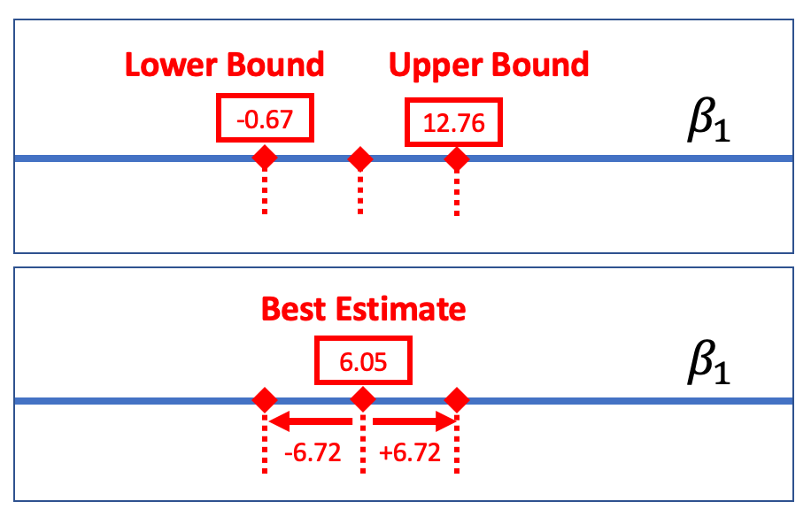
The margin of error is the distance between the upper bound and the sample estimate. In the case of the tipping experiment this would be \(12.76 - 6.05\), or $6.72. If we assume that the sampling distribution is symmetrical, the margin of error will be the same below the parameter estimate as it is above.
We can always calculate the margin of error by using confint() to get the upper bound of the confidence interval and then subtracting the sample estimate. But we can do a rough calculation of margin of error using the empirical rule. We learned in Chapter 6 that, according to the empirical rule, 95% of all observations under a normal curve fall within plus or minus 2 standard deviations from the mean.
Applying this rule to the sampling distribution, the picture below shows that the margin of error is approximately equal to two standard errors. If we start with a t-distribution centered at the sample \(b_1\), we would need to slide it up about two standard errors to reach the cutoff above which \(b_1\) (6.05) falls into the lower .025 tail.
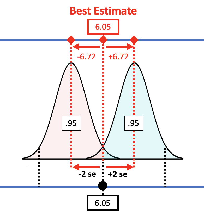
If you have an estimate of standard error, you can simply double it to get the approximate margin of error. If, for example, we use the standard error generated by R (3.33) for the condition model, the margin of error would be twice that, or 6.66. That’s pretty close to the margin of error we calculated from confint(): 6.72.
R uses the Central Limit Theorem to estimate standard error, but we also have other ways of getting the standard error. Using shuffle() to create the sampling distribution resulted in a slightly larger standard error of 3.5. If we double that, we get a margin of error of 7, slightly larger than the 6.66 we got using R’s estimate of standard error. In general, if the standard error is larger, the margin of error will be larger and so will the confidence interval.