2.6 Sampling From a Population
Turning variation in the world into data that we can analyze requires us to engage in two fundamental processes: measurement and sampling. Now that we’ve talked a little bit about measurement, let’s shift our attention to sampling.
There are two major decisions that underlie a sampling scheme. First, we must decide what to include in our universe of objects to be measured. This seems straightforward. But, it is not. When we decide which objects to include, we are saying, in effect, that these objects are all examples of the same category of things. (See the wonderful book, Willful Ignorance, for an in-depth discussion of this point.) This category of things can be referred to as the population. The population is usually conceptualized as large, which is why we study only a sample.
Let’s say we want to do a study of cocaine users to figure out the best ways to help them quit. What counts as a cocaine user? Someone who uses cocaine every day obviously would be included in the population. But what about someone who has used cocaine once? What about someone who used to frequently use cocaine but no longer does? You can see that our understanding of cocaine users will be impacted by how we define “cocaine user.”
Second, we must decide how to choose which objects from the defined population we actually want to select and measure. Most of the statistical techniques you will learn about in this course assume that your sample is independently and randomly chosen from the population you have defined.
Random Sampling
For a sample to be random, every object in the population must have an equal probability of being selected for the study. In practice, this is a hard standard to reach. But if we can’t have a truly random sample, we can at least try to feel confident that our sample is representative of the population we are trying to learn about.
For example, let’s say we want to measure how people from different countries rate their feelings of well-being. Which people should we ask? People from cities? Rural areas? Poor? Rich? What ages? Even though it might be difficult to select a truly random sample from the population, we might want to make sure that there are enough people in different age brackets, different socioeconomic status (SES), and different regions to be representative of that country.
Independent Sampling
Closely related to randomness is the concept of independence. Independence in the context of sampling means that the selection of one object for a study has no effect on the selection of another object; if the two are selected, they are selected independently, just by chance.
Like randomness, the assumption of independence is often violated in practice. For example, it might be convenient to sample two children from the same family for a study—think of all the time you’d save not having to go find yet another independently and randomly selected child!
But this presents a problem: if two children are from the same family, they also are likely to be similar to each other on whatever outcome variable we might be studying, or at least more similar than would a randomly selected pair. This lack of independence could lead us to draw erroneous conclusions from our data.
Sampling Variation
Every sample we take—especially if they are small samples—will vary. That is, samples will be different from one another. In addition, no sample will be perfectly representative of the population. This variation is referred to as sampling variation or sampling error. Similar to measurement error, sampling error can either be biased or unbiased.
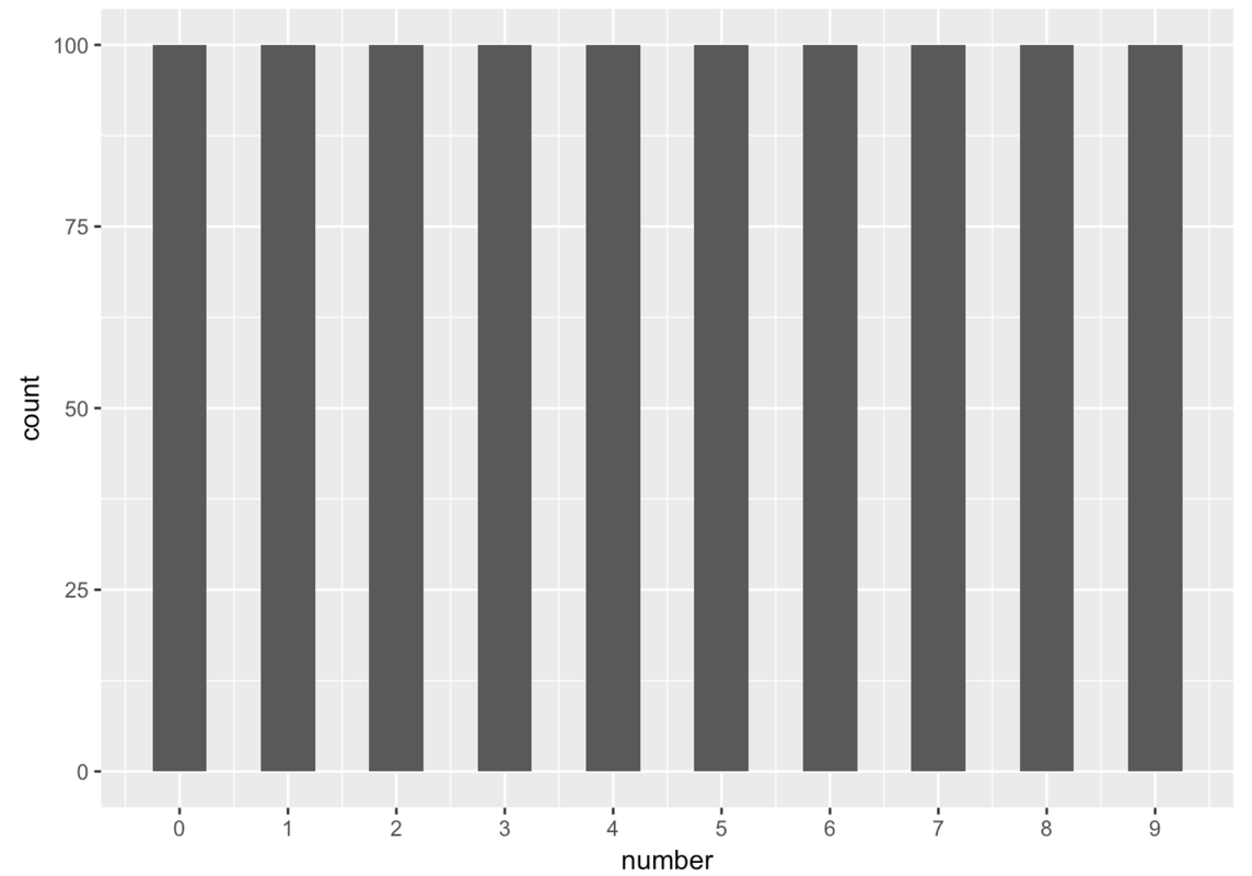
For example, we’ve created a vector called fake_pop (for fake population) that has 100 0s, 100 1s, 100 2s, 100 3s, and so on for the numbers 0 to 9. Here is a graph (called a histogram) that helps you see that there are 100 of each digit in this fake population.
Now let’s take a random sample of 10 numbers from fake_pop and save the result in a vector called random_sample. R provides a function for this, called sample().
Run the code to take a random sample of 10 numbers from fake_pop and save them in random_sample. We’ve also included some code to create a histogram but don’t worry about that part. We’ll build histograms together in Chapter 3.
require(coursekata)
fake_pop <- rep(0:9, each = 100)
# This takes a random sample of 10 numbers
# from fake_pop and saves them in random_sample
random_sample <- sample(fake_pop, 10)

# This makes a histogram of your sample
gf_histogram(~random_sample) %>%
    gf_refine(scale_x_continuous(breaks = 0:9))
random_sample <- sample(fake_pop, 10)

# this will make a histogram of your sample
gf_histogram(~random_sample) %>%
    gf_refine(scale_x_continuous(breaks = 0:9))
ex() %>% {
    check_object(., "random_sample")
    check_function(., "gf_histogram")
}You can run the R code above a few times to see a few different random samples. You’ll observe that these samples differ from each other and differ from the population they came from. Below we have depicted one example of a random sample of 10 numbers from fake_pop.
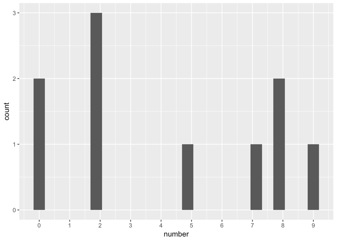
Notice that even a random sample won’t “look” just like the population it came from. This fundamental idea of sampling variation is a tough problem. We’re going to meet up with sampling variation a lot in statistics.
Bias in the context of sampling means that some objects in the population are more likely than others to be included in the sample even though there aren’t actually more of those objects in the population. This violates the assumptions of an independent random sample. Because of sampling variation, no sample will perfectly represent the population. But if we select independent random samples, we can at least know that our sample is unbiased—no more likely to be off in one direction than in another. So even though our random sample did not look just like the population, it was unbiased in that it wasn’t more likely to be off in a particular way (e.g., only sampling even numbers or large numbers).