12.8 The Logic of Inference with the Multivariate Model
Both F (and PRE) provide us ways to assess, with a single number, how well the multivariate model fits our data compared to the empty model. We have learned, in this case, that 54% of the variation in PriceK can be explained by our multivariate model, using both neighborhood and home size as predictors.
But our real interest is not in what is true about our data, but what is true about the Data Generating Process. One important reason that the data and the DGP may differ is sampling variation: samples from the same DGP will differ one to the next just based on randomness. “Statistical inference” refers to the process by which, using sampling distributions, we infer what is true in the DGP based on our models based on data.
In this book we have taken two approaches to inference: Model comparison, in which we try to decide which of two models is a better model of the DGP; and confidence intervals, in which we try to figure out what the true parameter might be based on the particular estimate we have created from our data. Let’s see how both of these play out in the context of multivariate models.
The Logic of Model Comparison
In model comparison we compare a more complex model of the DGP to a simpler one. Previously we compared a single-predictor model (more complex) to the empty model (simpler). We can use the same approach to compare the multivariate model of the DGP to the empty model. A sampling distribution of F is constructed based on the assumption that the empty model is true, and then the sample F from fitting the multivariate model to the data is evaluated in the context of that sampling distribution.
If the F is judged unlikely to have been generated by the empty model, the empty model is rejected in favor of the multivariate model. If the F is judged not unlikely to have been generated by the empty model, the empty model is retained. Let’s go through this in more detail below.
In the case of our multivariate model of PriceK, these are the two models that are being compared:
Complex: \(Y_i = \beta_0 + \beta_1X_{1i} + \beta_2X_{2i} + \epsilon_i\)
Simple: \(Y_i = \beta_0 + \epsilon_i\)
Note that in model comparison, we are always comparing two models, one complex and one simple. But complex and simple are relative terms. In the case of single-predictor models, the complex model is not as complex as the multivariate model, though it is still more complex than the empty model. The empty model, however, is the simplest of simple models.
Creating a Sampling Distribution of F Assuming the Empty Model
Before, with single-predictor models, we had just one explanatory variable (e.g., Neighborhood) in our model. We compared the neighborhood model to the empty model, which assumed that there was no relationship in the DGP between the outcome (PriceK) and the predictor (Neighborhood). Any such relationship in the data, therefore, was assumed to be completely the result of random chance.
In the table below, we have written the GLM notation for the neighborhood model and the empty model of the DGP as well as a snippet of R code that represents these two DGPs.
| Neighborhood model of the DGP | Empty model of the DGP |
|---|---|
\(Y_i = \beta_0 + \beta_1X_{1i} + \epsilon_i\)PriceK ~ Neighborhood
|
\(Y_i = \beta_0 + (0)X_{1i} + \epsilon_i\)shuffle(PriceK) ~ Neighborhood
|
Notice that we included the term \(X_{1i}\) in our representation of the empty model, but replaced the \(\beta_1\) with a 0. This is a way of indicating that we didn’t just write a model without Neighborhood, but instead a model in which the effect of Neighborhood is constrained to be 0. We mimicked this DGP in R by using the shuffle() function before PriceK. Now there is no relationship (except a random one) between PriceK and Neighborhood.
In the table below, we have written the GLM notation for the multivariate and empty models of the DGP (along with a bit of R code).
| Multivariate model of the DGP | Empty model of that DGP |
|---|---|
\(Y_i = \beta_0 + \beta_1X_{1i} + \beta_2X_{2i} + \epsilon_i\)PriceK ~ Neighborhood + HomeSizeK
|
\(Y_i = \beta_0 + (0)X_{1i} + (0)X_{2i} + \epsilon_i\)shuffle(PriceK) ~ Neighborhood + HomeSizeK
|
With single-predictor models we could shuffle either the outcome or the predictor variable; the result would be the same. With multivariate models we will shuffle the outcome variable because we want to leave the relationship between Neighborhood and HomeSizeK intact, while breaking the relationship of both variables to PriceK.
We can use this random DGP to generate a sampling distribution of Fs, and then compare the sample F obtained by fitting the multivariate model to our data against this sampling distribution.
We can calculate a p-value that will tell us how likely an F as extreme as the one we observed would be to have come from a DGP in which the empty model is true. If it is unlikely (and we can define “unlikely” as less than .05), then we can reject the empty model in favor of our multivariate model.
Notice that this is the same logic of hypothesis testing and almost the same R code we used with single-predictor models. The only difference is that shuffling the outcome now breaks its relationship to multiple explanatory variables instead of just one.
Below we have written code to calculate the sample f() for the multivariate model. Modify the code to shuffle() the outcome variable.
require(coursekata)

# delete when coursekata-r updated
Smallville <- read.csv("https://docs.google.com/spreadsheets/d/e/2PACX-1vTUey0jLO87REoQRRGJeG43iN1lkds_lmcnke1fuvS7BTb62jLucJ4WeIt7RW4mfRpk8n5iYvNmgf5l/pub?gid=1024959265&single=true&output=csv")
Smallville$Neighborhood <- factor(Smallville$Neighborhood)
Smallville$HasFireplace <- factor(Smallville$HasFireplace)
# modify this to generate an F from the empty model of the DGP
f(PriceK~ Neighborhood + HomeSizeK, data = Smallville)
f(shuffle(PriceK) ~ Neighborhood + HomeSizeK, data = Smallville)
# temporary SCT
ex() %>% check_error()From just a few shuffles, it seems like it would be rare for a DGP in which the empty model is true to produce an F as large as 17. It might be possible, but it doesn’t look likely. We have only looked at a few Fs, however. Let’s see what else we can learn by creating a sampling distribution of 1000 shuffled Fs.
require(coursekata)

# delete when coursekata-r updated
Smallville <- read.csv("https://docs.google.com/spreadsheets/d/e/2PACX-1vTUey0jLO87REoQRRGJeG43iN1lkds_lmcnke1fuvS7BTb62jLucJ4WeIt7RW4mfRpk8n5iYvNmgf5l/pub?gid=1024959265&single=true&output=csv")
Smallville$Neighborhood <- factor(Smallville$Neighborhood)
Smallville$HasFireplace <- factor(Smallville$HasFireplace)
# add do() to generate a sampling distribution of 1000 Fs
# from the empty model of the DGP
sdof <- f(shuffle(PriceK) ~ Neighborhood + HomeSizeK, data = Smallville)

# this will depict the sdof in a histogram
gf_histogram(~ f, data = sdof)
sdof <- do(1000) * f(shuffle(PriceK)~ Neighborhood + HomeSizeK, data = Smallville)
gf_histogram(~ f, data = sdof)
# temporary SCT
ex() %>% check_error()
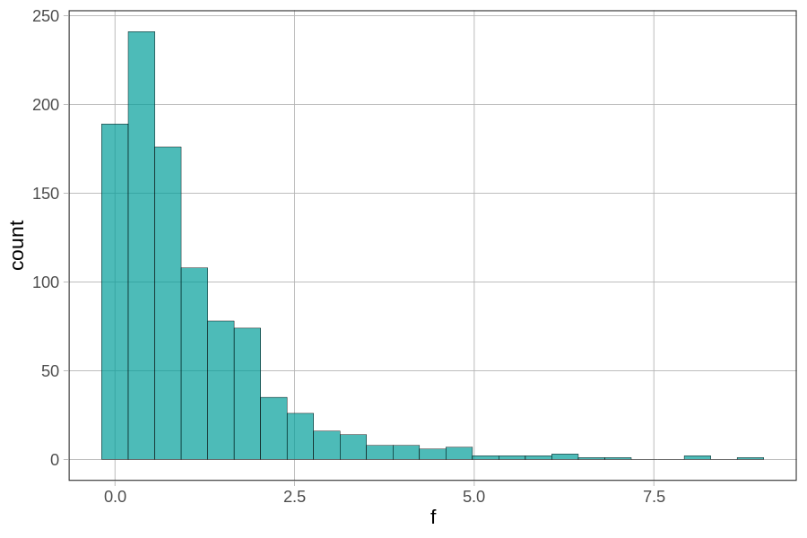
Notice that the sampling distribution is bounded at the lower end by 0, and is skewed, with a long tail to the right. We can see by the scale on the x-axis that none of the 1000 randomly generated Fs were as large as the sample F of 17. The highest one, in fact, appears to be about 8 or so.