6.4 Standard Deviation
The standard deviation (written as \(s\)) is simply the square root of the variance. We generally prefer thinking about error in terms of standard deviation because it yields a number that makes sense using the original scale of measurement. So, for example, if you were modeling weight in pounds, variance would express the error in squared pounds (not something we are used to thinking about), whereas standard deviation would express the error in pounds.
Here are two formulas that represent the standard deviation:
\[s = \sqrt{s^2}\]
\[\sqrt{\frac{\sum_{i=1}^n (Y_i-\bar{Y})^2}{n-1}}\]
To calculate standard deviation in R, we use sd(). Here is how to calculate the standard deviation of our Thumb data from TinyFingers.
sd(TinyFingers$Thumb)[1] 4.049691There are actually a few different ways you can get the standard deviation for a variable. One is the function sd(), obviously. But you can also square root the variance with a combination of the functions sqrt() and var(). Yet another, and possibly more useful, way is to use good old favstats(). Try all three of these methods to calculate the standard deviation of Thumb from the larger Fingers data frame.
require(coursekata)
empty_model <- lm(Thumb ~ NULL, data = Fingers)
# calculate the standard deviation of Thumb from Fingers with sd()

# calculate the standard deviation with sqrt() and var()

# calculate the standard deviation with favstats()
sd(Fingers$Thumb)
sqrt(var(Fingers$Thumb))
favstats(~Thumb, data = Fingers)
ex() %>% {
    check_function(., "sd") %>% check_result() %>% check_equal()
    check_function(., "sqrt") %>% check_result() %>% check_equal()
    check_function(., "favstats") %>% check_result() %>% check_equal()
}[1] 8.726695[1] 8.726695 min Q1 median Q3 max mean sd n missing
39 55 60 65 90 60.10366 8.726695 157 0Sum of Squares, Variance, and Standard Deviation
We have discussed three ways of quantifying error around our model. All start with residuals, but they aggregate those residuals in different ways to summarize total error.
All of them are minimized at the mean, and so all are useful when the mean is the model for a quantitative variable.
Thinking About Quantifying Error in MindsetMatters
Below is a histogram of amount of weight lost (PoundsLost) by each of the 75 housekeepers in the MindsetMatters data frame.
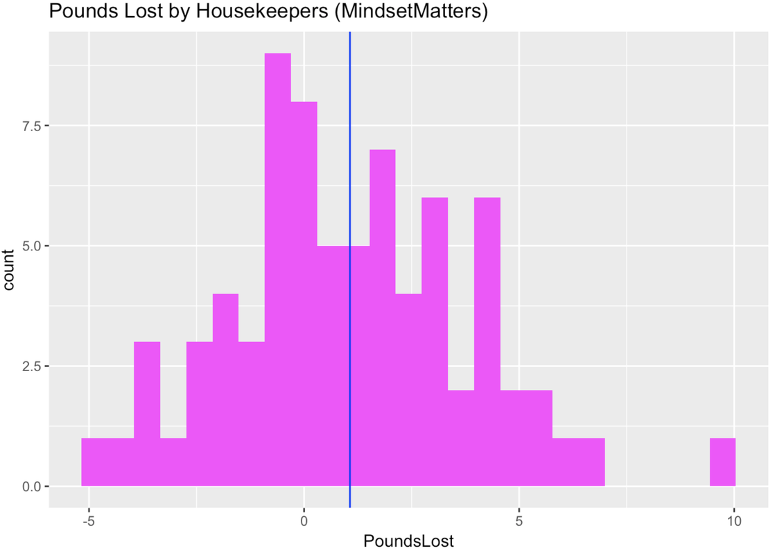
Use R to create an empty model of PoundsLost. Call it empty_model. Then find the SS, variance, and standard deviation around this model.
require(coursekata)
MindsetMatters$PoundsLost <- MindsetMatters$Wt - MindsetMatters$Wt2
# create an empty model of PoundsLost from MindsetMatters
empty_model <-

# find SS, var, and sd
# there are multiple correct solutions
empty_model <- lm(PoundsLost ~ NULL, data = MindsetMatters)
sum(resid(empty_model)^2)
var(MindsetMatters$PoundsLost)
sd(MindsetMatters$PoundsLost)
ex() %>% {
    check_object(., "empty_model") %>% check_equal()
    check_output(., 556.7)
    check_output(., 7.52)
    check_output(., 2.74)
}There are multiple ways to compute these in R, but here is one set of possible outputs.
Analysis of Variance Table (Type III SS)
Model: PoundsLost ~ NULL

                             SS  df    MS   F PRE   p
----- ----------------- ------- --- ----- --- --- ---
Model (error reduced) |     --- ---   --- --- --- ---
Error (from model)    |     --- ---   --- --- --- ---
----- ----------------- ------- --- ----- --- --- ---
Total (empty model)   | 556.727  74 7.523
[1] 7.523333[1] 2.74287SS: 556.7267Variance: 7.523333Standard Deviation: 2.74287Notation for Mean, Variance, and Standard Deviation
Finally, we also use different symbols to represent the variance and standard deviation of a sample, on one hand, and the population (or DGP), on the other. Sample statistics are also called estimates because they are our best estimates of the DGP parameters. We have summarized these symbols in the table below (pronunciations for symbols are in parentheses).
| Sample (or estimate) | DGP (or population) | |
|---|---|---|
| Mean | \(\bar{Y}\) (y bar) | \(\mu\) (mu) |
| Variance | \(s^2\) (s squared) | \(\sigma^2\) (sigma squared) |
| Standard Deviation | \(s\) (s) | \(\sigma\) (sigma) |
Variance is the mean squared error around the empty model. It is an average of the squared deviations from the mean. In tables, it may be shortened to be “mean square” or “MSE”. You now know that just means variance. Remember in the output (see below) from the supernova() function the column headed “MS”? That is, in fact, the variance.
supernova(empty_model)Analysis of Variance Table (Type III SS)
Model: Thumb ~ NULL
SS df MS F PRE p
----- ----------------- --------- --- ------ --- --- ---
Model (error reduced) | --- --- --- --- --- ---
Error (from model) | --- --- --- --- --- ---
----- ----------------- --------- --- ------ --- --- ---
Total (empty model) | 11880.211 156 76.155 var(Fingers$Thumb)[1] 76.1552