Chapter 13 - Multivariate Model Comparisons
13.1 Targeted Model Comparisons
Model comparisons always involve comparing a complex model to a simple model. So far, we have focused on comparing the full multivariate model, represented by the word equation PriceK= Neighborhood + HomeSizeK + Error, to the empty model, represented by PriceK= Mean + Error.
We can write these models of the DGP in GLM notation like this:
Complex: \(PriceK_i = \beta_0 + \beta_1NeighborhoodEastside_{i} + \beta_2HomeSizeK_{i} + \epsilon_i\)
Simple: \(PriceK_i = \beta_0 + \epsilon_i\)
From this model comparison we have concluded that the complex model does a significantly better job explaining variation in PriceK in the DGP than does the simple model. But this comparison doesn’t answer all of the questions we might have. For example, are both predictor variables necessary? Or is one actually all you need to be an adequate model of the DGP and to make good predictions?
To answer questions like this we will want to make more targeted model comparisons, and in particular those in which the complex and simple models differ by only one parameter. The models we compared above differed by two parameters: the multivariate model included both Neighborhood and HomeSizeK, whereas the empty model included neither.
What would be more useful, perhaps, is to compare a model with both Neighborhood and HomeSizeK to one with only Neighborhood. In this way we could find out if adding HomeSizeK to the model reduces error significantly above and beyond the amount error is reduced by just the Neighborhood model. These models differ by just one parameter: HomeSizeK.
The comparison between a model including both Neighborhood and HomeSizeK to one that includes only Neighborhood could be represented in GLM notation like this:
Complex: \(\beta_0 + \beta_1NeighborhoodEastside_{i} + \beta_2HomeSizeK_{i} + \epsilon_i\)
Simple: \(\beta_0 + \beta_1NeighborhoodEastside_{i} + \epsilon_i\)
Notice that the simple model in this case is not the empty model; it’s just simpler than the complex model. It’s actually just the single-predictor Neighborhood model that we have seen before. The complex and simple models differ in just one way: the inclusion or exclusion of \(\beta_2HomeSizeK_{i}\). By comparing these two models, we can see the unique contribution of HomeSizeK.
If we compare the error from these two models, we can see how much error is reduced by including HomeSizeK in the model over and above the amount reduced by the single-predictor Neighborhood model. We will use sums of squares and PRE to make this comparison in our data.
Representing Targeted Model Comparisons with Venn Diagrams
Let’s return to our Venn diagram to think about how the complex model (the multivariate one) will compare against our simple model (the single-predictor model using Neighborhood).
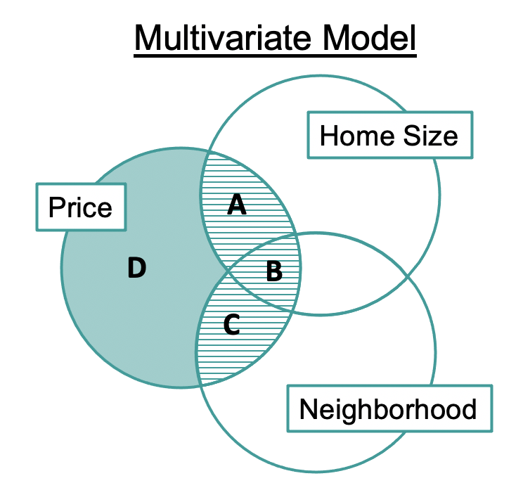
The difference between the complex and simple models is the inclusion/exclusion of HomeSizeK. The difference in the sum of squared error reduced by the complex model (A+B+C) and simple model (B+C) is the region labeled A. That is the reduction in error that can be uniquely attributed to HomeSizeK.
The sum of squares represented by region A will tell us how much variation in PriceK is explained by HomeSizeK after explaining as much as possible with Neighborhood.