3.5 The Back and Forth Between Data and the DGP
Data analysis involves working back-and-forth between the data distribution, on one hand, and our best guess of what the population distribution looks like, on the other. We need to keep this in mind in order to understand the DGP that might have produced the variation in the population and thus the variation we see in our data.
As you learn to think like a statistician, it helps to understand the two key moves that you will use as part of this back-and-forth.
Looking at a distribution of data, you try to imagine what the population distribution might look like, and what processes might have produced such a distribution. We will call this a bottom-up strategy as we move from concrete data to the more unknown, abstract DGP.
Thinking about the DGP, and all that you know about the world, you try to imagine what the data distribution should look like, if your theory of the DGP is true. We will call this the top-down strategy as we move from our ideas about the DGP to predicting actual data.
We illustrated the bottom-up move above when we looked at the distribution of wait times at a bus stop and tried to imagine the process that generated it. The top-down move would come into play if we asked: what if buses worked differently? What if, instead of following schedules, a new bus left the stop every time 10 people were waiting there? What would the distribution of wait times look like if this were the case?
You can probably imagine a few different possibilities. That’s great! Having some expectations about the DGP (whether they are right or wrong) helps us interpret any data that we actually do collect.
Both of these moves are important. Sometimes we have no clue what the DGP is, so we must use the bottom-up strategy looking for clues in the data. Based on these clues, we generate hypotheses about the DGP.
But other times, we have some well-formulated ideas of the DGP and we want to test our ideas by looking at the data distribution. In the top-down move we say: if our theory is correct, what should the data distribution look like? If it looks like we predict, our theory is supported. But if it doesn’t, we can be pretty sure we are wrong about the DGP.
When We Know the DGP: The Case of Rolling Dice
Our understanding of the DGP is usually quite fuzzy and imperfect, and often downright wrong. But there are some DGPs we have a good understanding of. Some well-known examples of random processes are those associated with flipping coins or rolling dice.
Randomness turns out to be an important DGP for the field of statistics. We often ask, for example, could the distribution we see in our data be the result of purely random processes? Answering this question requires some facility with the top-down move discussed above.
If the process is random, what would the distribution of data look like? (Note the importance of the word “if” in thinking statistically.) Because random models are well understood, it is easier to answer this question for randomness than it is for other causal processes.
Dice provide a familiar model for thinking about random processes. They also provide another example for thinking about the related concepts of sample, population and DGP. In most research we are trying to understand things we don’t already know, so we go bottom-up as we start with a sample and try to guess what the DGP might be like. With dice we have the luxury of going top-down, starting with the DGP, simply because we know what it is.
We have a sense that the process is somehow random, that each number has a roughly equal likelihood of coming up. And even though factors such as how we hold the dice or throw the dice or the wind conditions might play a role in any individual throw, we still have a sense that over the long term, with many many rolls, we would end up with a roughly equal number of 1s, 2s, 3s, 4s, 5s, and 6s.
What is the DGP in this case? Even if we roll a die only once, we still assume that the DGP is operating fully. It is a random process in which each of the six possible outcomes (the numbers on the die) has a one out of six chance of coming up.
The population is what the distribution of dice rolls would look like if the DGP were to operate repeatedly over a long period of time. We don’t know exactly how many times one would have to roll a die to create a population; it could even be an infinite number of times. But we do know that, in the long run, the population distribution produced by this DGP would look something like this (see sketch below).
Most people imagine that if we ran this DGP (die rolling) for a long time, the resulting population distribution would be uniform (such as the sketch above), with each of the digits from 1 to 6 having an equal probability of occurring. This expectation is based on our understanding of how dice rolls work.
Investigating Samples From a Known DGP
Knowing what the DGP is (as in the case of dice) gives us a chance to investigate the relationship between samples and populations. Let’s say we take a small sample of 12 students and ask them each to roll a die one time.
Even when we know what the true DGP is, we will rarely see a sample distribution—especially for a small sample—that mirrors the population distribution. There is always a little fluctuation due to natural variation from one sample to the next. We call this kind of fluctuation sampling variation.
How much fluctuation? We can get a sense of this by doing a simulation. Let’s use R to mock up a DGP that models the one for the dice.
First, let’s create a simulated die in R. We’ll create a vector called model_pop. It represents a die in the sense that each of the numbers (1 to 6) appears only once, just like an actual die. We will use it to model the population (hence the name model_pop).
model_pop <- c(1, 2, 3, 4, 5, 6)The function gf_histogram() can also make a histogram out of a vector, like this:
gf_histogram(~ model_pop)Note that it doesn’t have the data = part because model_pop is not in a data frame. (gf_histogram is flexible because it can graph vectors or variables in a data frame. Notice that gf_histogram() always expects a ~, then the vector or variable name. In this case, we are just graphing a vector.)
Write code to create a density histogram of model_pop with just six bins (we don’t need the default 30 bins because there are only six possible numbers). Feel free to play with colors using the arguments color and fill.
require(coursekata)
# This creates our model population
model_pop <- 1:6

# Write code to create a relative frequency histogram of our model population.
# Remember to include bins as an argument.
# This creates our model population
model_pop <- 1:6

# Write code to create a relative frequency histogram of our model population.
# Remember to include bins as an argument.
# gf_dhistogram(~ model_pop, color = "black", bins = 6)
ex() %>% {
    check_object(., "model_pop") %>% check_equal()
    override_solution_code(.,
        'gf_dhistogram(~ model_pop, color = "black", bins = 6)'
    ) %>%
        check_function(., "gf_dhistogram") %>% {
            check_arg(., "object") %>% check_equal()
            check_arg(., "bins") %>% check_equal()
        }
}
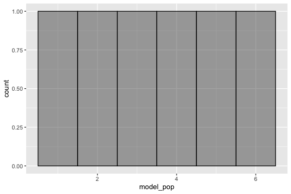
You shouldn’t be surprised at the shape of this density histogram. It is a perfect, uniform distribution in which each of the numbers 1 to 6 has an equal probability of occurring. This density histogram can be thought of as both a model of the DGP, and a model of what the population distribution would look like in the long run.
Now, we’ll simulate rolling a die once by taking a single sample from the numbers 1 to 6 from our model population. We can use the R command sample() which we have used before for this purpose.
sample(model_pop, 1)This is telling R to randomly take one number from the numbers in model_pop, of which there are six. We ran it and got the following output.
[1] 2Turns out our simulated die rolled a 2.
We could type this out 12 times to simulate getting a sample of 12 die rolls. Or we could use the do() command to do this 12 times.
do(12) * sample(model_pop, 1) sample
1 4
2 2
3 6
4 6
5 1
6 6
7 3
8 4
9 4
10 2
11 5
12 2Or, we could use the command resample() to sample in the same way 12 times.
resample(model_pop, 12) [1] 3 6 6 2 3 1 4 3 6 1 3 3You might be wondering, can’t we just type 12 into sample(model_pop, 12)? Would that accomplish the same thing as resample(model_pop, 12)? Run the code to try both of them here.
require(coursekata)
allow_solution_error()
; # semicolon must be here for allow_solution_error to work
# TODO: CKC-38
model_pop <- 1:6

# This samples the same way 12 times
resample(model_pop, 12)

# Will this accomplish the same thing?
# Do not change the code --- just submit it
sample(model_pop, 12)
success_msg("This code is supposed to throw an error. You can read it in the Console tab.")Sampling With and Without Replacement
When we try it with sample() we get an error message! (Sorry, we set you up.) This is because the command sample() will take a sample, and then remove the number that it sampled. Then it samples again from the remaining numbers. This is called sampling without replacement.
Even though we tell R to sample 12 times, there are only six numbers, which means that it will run out of numbers to sample! This is why the error message says “cannot take a sample larger than the population.”
The command resample() works a different way; it samples with replacement, which means that once it samples one number from the population of six, it replaces it so that it can be sampled again.
Whereas sampling without replacement—sample()—can only go on until you run out of numbers to sample, sampling with replacement—resample()—could, theoretically, go on forever.