9.2 Constructing a Sampling Distribution
The Tipping Study: Again
We have introduced two ideas that probably sound quite abstract at this point: sampling distribution and rejecting the empty model. To make these ideas more concrete, let’s revisit the tipping study that we explored previously.
In the tipping study (for reference, here you can download the article for the tipping study (PDF, 419KB)), you may recall, researchers examined whether putting hand-drawn smiley faces on the back of a restaurant check would cause customers to give higher tips to their server. Each table was randomly assigned to receive their check with either a smiley face on it or not. The outcome variable was the amount of tip left by each table.
Here’s a random sample of six observations from the data frame TipExperiment:
sample(TipExperiment, 6) TableID Tip Condition
20 20 20 Control
26 26 44 Smiley Face
19 19 21 Control
15 15 25 Control
25 25 47 Smiley Face
18 18 21 ControlThe researchers want to explore the hypothesis that Tips = Condition + Other Stuff. The GLM notation for this two-group model would be:
\[Y_{i}=b_{0}+b_{1}X_{i}+e_{i}\]
in which \(X_{i}\) represents whether a table was in the Smiley Face condition or not (coded 0 for Control tables and 1 for Smiley Face tables). The parameter estimate the researchers are most interested in is \(b_{1}\) which represents the difference in average tips between the two conditions. This is our best estimate of \(\beta_{1}\), the true effect of adding a smiley face to checks in the DGP.
Before we remind ourselves of what the results of the study look like, let’s imagine what we would expect to see if a particular model of the DGP were true. For example, if there is a benefit of drawing smiley faces in the DGP (i.e., if \(\beta_1\) is a positive value), we might expect that samples from such a DGP would have positive \(b_1\)s on average.
Although we couldn’t predict any single \(b_1\) that comes from a particular DGP, we can make predictions about the average \(b_1\) that would be generated from multiple random samples. On average, the \(b_1\)s would tend to resemble the parent \(\beta_1\) from which they come. So a negative \(\beta_1\) would tend to produce negative \(b_1\)s, a positive \(\beta_1\), positive \(b_1\)s.
The empty model is a special case in which \(\beta_1=0\). If the empty model is true it means that drawing a smiley face has no effect on how much tables tip. The \(b_1\)s generated by multiple random samples from a DGP in which \(\beta_1=0\) would tend to be close to 0, but they wouldn’t necessarily be exactly 0. We can construct a sampling distribution to find out if our sample \(b_1\) could have been generated by the empty model.
Constructing a Sampling Distribution Assuming the Empty Model
Let’s engage in some hypothetical thinking. If there were no effect of drawing smiley faces, these tables would have tipped the same amount whether they were randomly assigned to one group or the other. (We discussed this previously on page 7.8.)
One great thing about modern statistics and data science is that we are not limited to simply imagining what the \(b_1\)s would look like if there were no effect of smiley face in the DGP. We can actually use R to simulate this DGP, in which \(\beta_1=0\). Remember, empty model, \(\beta_1=0\), and “no effect” all mean the same thing: none of the variation across tables in tips is caused by drawing smiley faces.
We can use the shuffle() function to simulate this hypothetical situation, randomly assigning each Tip (representing each table) in the data frame to be in either the Smiley Face or Control condition.
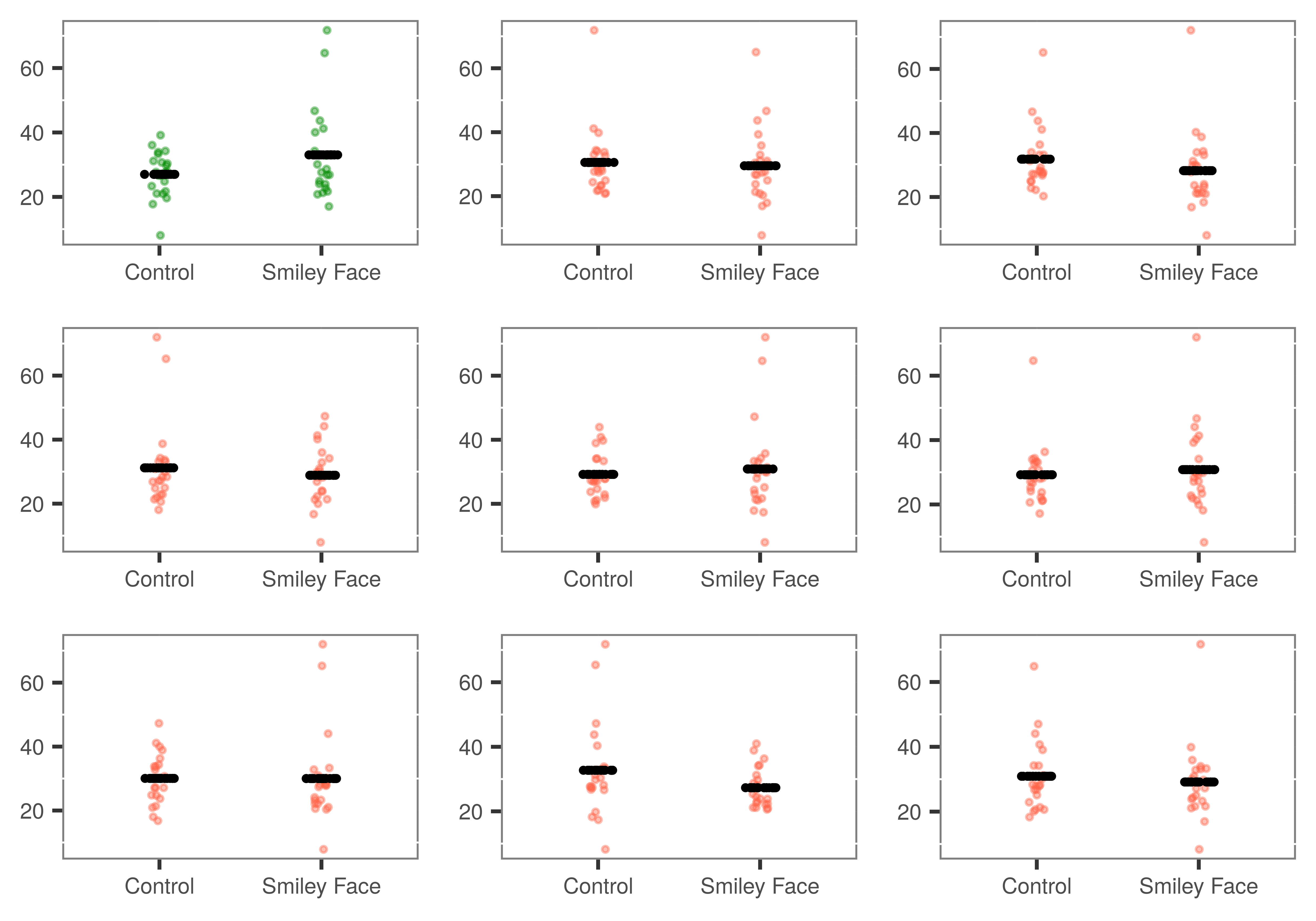
The figure below shows the real sample data (the green jitter plot in the upper left) along with 8 different random pairings of tips (for each table) with conditions. For each randomization, we have plotted the average tip (the black lines) for each of the newly-randomized groups.
The code below will generate the best fitting \(b_1\) from a single shuffle of the data. You can run it a few times just to see that each shuffle results in a different \(b_1\). Now modify the code (by adding the do() function) to simulate 1000 \(b_1\)s, one for each shuffle of the data.
require(coursekata)
b1(shuffle(Tip) ~ Condition, data = TipExperiment)
do(1000) * b1(shuffle(Tip) ~ Condition, data = TipExperiment)
ex() %>%
       check_function("do") %>%
       check_arg("object") %>%
check_equal()Woah, that’s a lot of numbers! We can notice a few things, though, just by looking at the first few numbers on the list. We can see, for example, that the \(b_1\)s vary each time we shuffle and calculate a new \(b_1\). Even though we couldn’t have predicted whether the first \(b_1\) would be positive or negative, we knew that some of the \(b_1\)s would be positive and some would be negative.
Even though the 1000 numbers generated by R seem similar to a distribution of sample data, they are different in two important ways. First, they are not based on measurement of a variable but on a random generation process; the numbers are generated by R. Second, and most critical, each number (i.e., each \(b_1\)) represents a parameter estimate, not an individual observation.
Distributions that share these features are called sampling distributions. They aren’t data, though, as in this case, they can be constructed using data. But whereas you have only one sample of data for a given study, sampling distributions are simulations of what it might look like if you had done the same study multiple times.
A sampling distribution is a distribution of parameter estimates (or sample statistics) computed on randomly generated samples of a given size.
Sampling distributions let us see what the sampling variation across multiple studies might look like if you were to repeat the same data collection process (i.e., selecting a random sample, or randomly assigning cases to conditions) a very large number of times.