Chapter 11: Parameter Estimation and Confidence Intervals
11.1 From Hypothesis Testing to Confidence Intervals
In Chapters 9 and 10 our focus has been on using data to evaluate the empty model of the DGP. We created sampling distributions based on the empty model, then asked whether we could reject the empty model based on our data. If the evidence was not strong enough to justify rejecting the empty model, we would keep the empty model as a plausible model. If we rejected the empty model, on the other hand, we would adopt the complex model we had made to fit the data.
The problem with this approach is that it only considers two possible models of the DGP, one in which \(\beta_1\) is 0, and one in which \(\beta_1\) is the same as the \(b_1\) estimate (e.g., $6.05 in the tipping study). But deep down, we know that both models might be wrong.
In the tipping study, we failed to reject the empty model, even though the tables who got the smiley faces tipped $6.05 more than the other tables. This evidence was not strong enough to cause us to reject the empty model, but does that mean the true \(\beta_1\) is actually 0? It’s possible. But in fact, there are many possible values of \(\beta_1\) that would be consistent with the data.
In this chapter we will use the same sampling distributions we have been using for model comparison, but use them in a more flexible way to ask a different question: What is the range of possible values for the parameter we are trying to estimate? In the case of the tipping study, it’s nice to know that the true \(\beta_1\) in the DGP might be 0, but what else might it be? If our best estimate, based on the data, is $6.05, we want to know how accurate that estimate might be and how much uncertainty we should have about the estimate.
Reviewing the Null Hypothesis Test Using \(b_1\)
Let’s start by reviewing the logic behind the null hypothesis test, i.e., the way we evaluated the empty model. As shown in the picture below, we start by imagining a world where the empty model is true, where there is no effect of smiley face on Tip. We represent this idea by putting a 0 in the red box on the upper blue line, which is where we put our hypotheses about the true \(\beta_1\) in the DGP.
It is important to remember that we don’t know if \(\beta_1 = 0\) or not. We are simply hypothesizing that it’s 0 so that we can then work out the implications that might follow from such a world. Later we will hypothesize other values of \(\beta_1\), moving the red box right and left to represent larger or smaller values of \(\beta_1\).
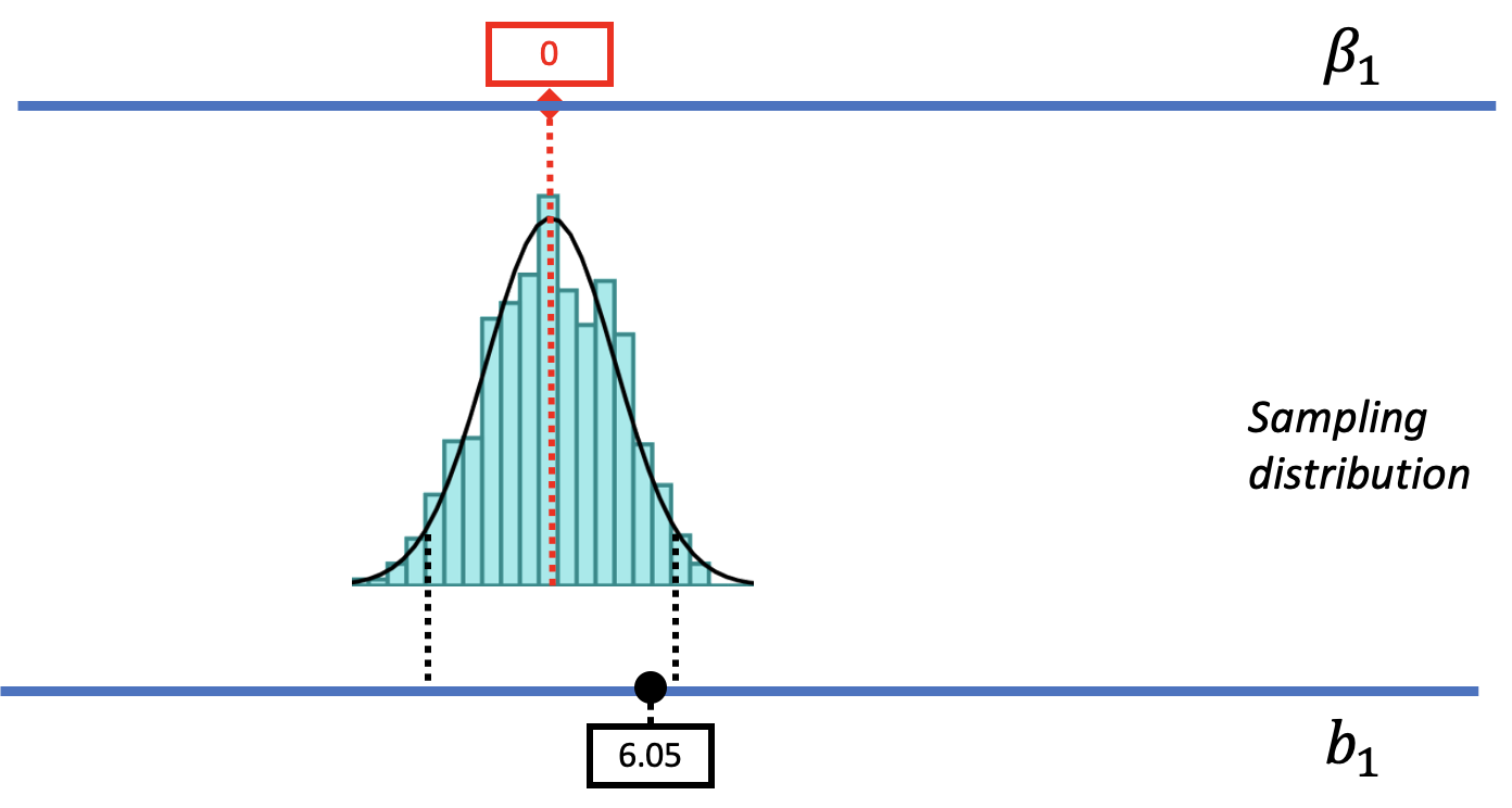
Based on the assumption that \(\beta_1 = 0\), we used shuffle() to create a sampling distribution (shown as a light blue histogram in the figure above) that shows us the variation in sample \(b_1\)s that would be expected to occur just by chance alone if the empty model is true. (This sampling distribution is approximately normal in shape, and is usually modeled with the t-distribution. We show the t-distribution as a smooth curve overlaid on the histogram.)
Having created a sampling distribution, we next located the sample \(b_1\) (6.05) in relation to the sampling distribution. The sample \(b_1\), which we have represented with a black dot on the bottom blue line, which represents the data, is not something we imagine or hypothesize. It’s the parameter estimate the researchers calculated from the sample data. It is fixed and can’t be moved.
Because the sample \(b_1\) did not fall in the .05 outer tails (our alpha criterion) of this sampling distribution, we decided to not reject the empty model (or null hypothesis). The p-value was approximately .08, meaning that if the empty model were true there would be a .08 chance of getting a sample as extreme as the sample \(b_1\) just by chance.
Thinking With Sampling Distributions
Up to now, we have centered all of our thinking with sampling distributions around the empty model. In Chapters 9 and 10, we always started by assuming that \(\beta_1\) is 0 and then went on to make sampling distributions based on this assumption. In this chapter we will move beyond the empty model and consider other models that could have produced the sample \(b_1\).
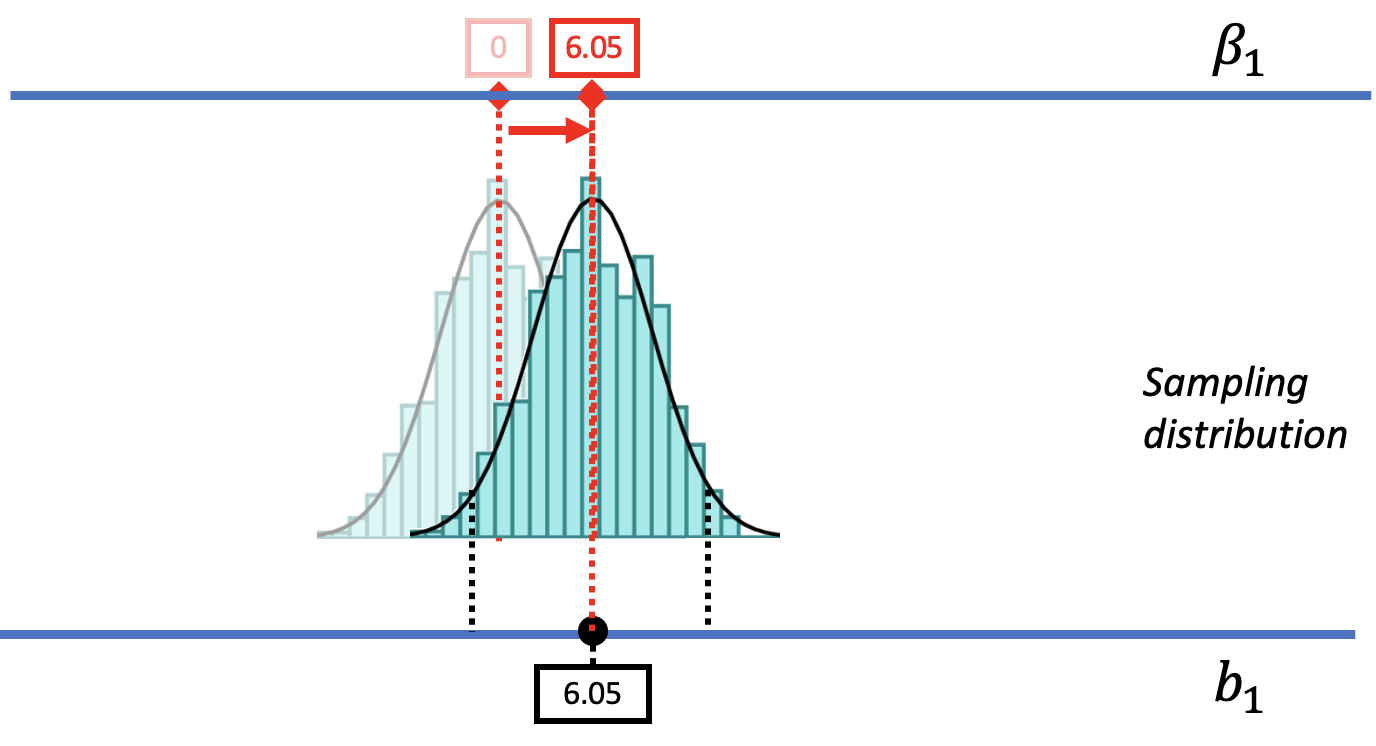
Our basic strategy is illustrated in the animated gif below. We start with the same sampling distribution we constructed based on the empty model. But then, using our hypothetical thinking skills, we mentally move the sampling distribution up and down along the number line, imagining different possible values of \(\beta_1\).
As we begin thinking about alternative models of the DGP, we will assume that the shape and spread of the sampling distribution stays constant across different hypothesized values of \(\beta_1\). By making these assumptions, it makes it possible for us to use a sampling distribution created based on one particular DGP (e.g., the empty model) for other DGPs up and down the scale. Later we will provide more justification for this assumption, but for now just go with us!
As we mentally move the sampling distribution up and down the measurement scale we consider different possible values of \(\beta_1\). For each of these possible values we ask the same question we asked using the sampling distribution centered at a \(\beta_1\) of 0: Given the new hypothesized value of \(\beta_1\), is such a DGP likely to generate our sample \(b_1\)?
Let us show you what we mean. In the figure below we have moved the sampling distribution we constructed based on the empty model for the tipping study up (to the right) until it is centered at a DGP where \(\beta_1=6.05\). We now pose the question, “If the true \(\beta_1\) is $6.05, is our sample \(b_1\) of $6.05 likely?
|
|
We saw before that a DGP in which \(\beta_1=0\) could produce the observed sample \(b_1\) of $6.05. That was our reason for not rejecting the empty model. But that does not mean the true \(\beta_1\) in the DGP is actually 0. The pictures above show it’s also possible that the true \(\beta_1\) is $6.05! And $6.05 was, after all, the best-fitting estimate of \(\beta_1\) based on the data.
From our musings so far, we can see that \(\beta_1\) could be 0 or it could be $6.05. But these are just two of the many possible DGPs that could have produced the sample estimate of $6.05. Once we start imagining different possible DGPs, and the sampling distributions each would generate, we will see more and more possibilities.
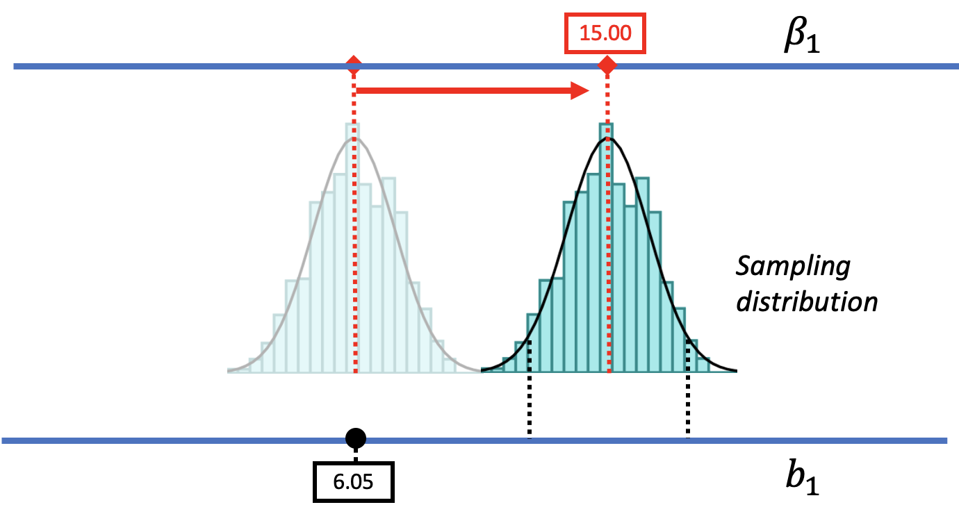
But using this strategy, we can also rule out some possibilities. There are values of \(\beta_1\) that are not likely to produce the sample estimate. Imagine a DGP with a \(\beta_1\) a lot larger than $6.05; for example, a world where the true difference between groups is 15.00. To represent this world, we could slide the DGP as well as its corresponding sampling distribution further to the right (see the picture below).
Such a DGP could produce a variety of samples. But notice that the sample \(b_1\) of $6.05 is no longer in the middle .95 region – now it’s in the lower unlikely tail. We could say, therefore, that a DGP with \(\beta_1=15.00\) is unlikely to have generated the sample \(b_1\) because $6.05 is much lower than most of the \(b_1\)s generated by this DGP.
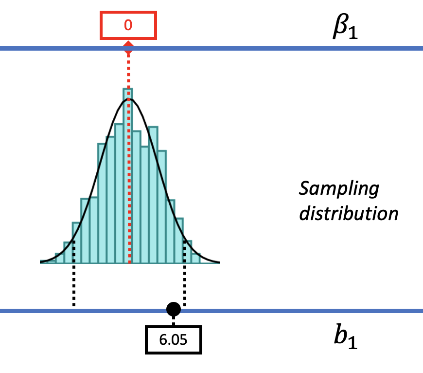
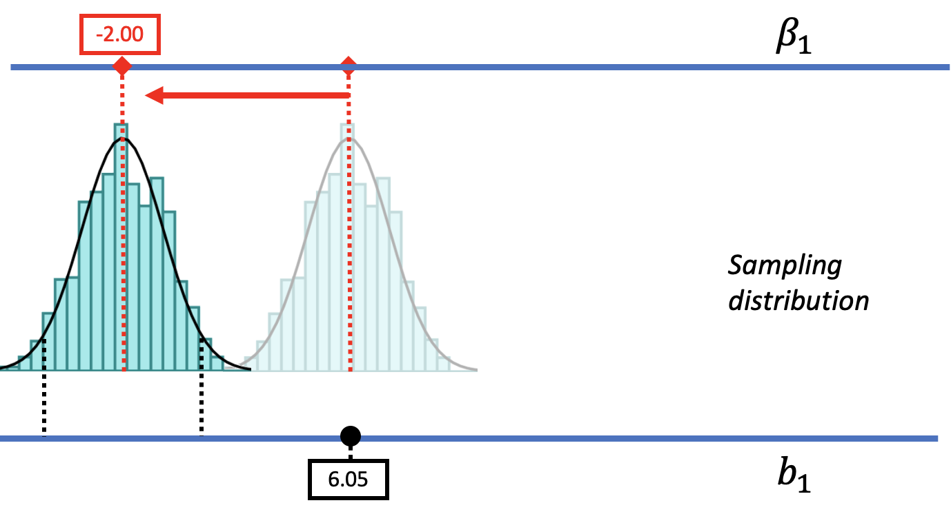
By the same logic, if we slide the sampling distribution far down to the left (as in the figure below), we can see that it is unlikely that the \(b_1\) of $6.05 came from a DGP with a \(\beta_1\) as low as -2.00. By sliding the sampling distribution left and right, we can begin to see the range of possible \(\beta_1\)s that could have generated our sample \(b_1\).
The Basic Idea Behind Confidence Intervals
If we extend this logic just a bit, we will be able to find the range of \(\beta_1\)s that would be likely to produce the sample \(b_1\); this is the basic idea behind confidence intervals. We’re using the word “likely” to mean that the sample \(b_1\) would be part of the middle .95 most likely samples from these DGPs.
Instead of answering a yes/no question as to whether we should reject the empty model or not, confidence intervals allow us to quantify the variation in a sample estimate and make statements such as, “We are 95% confident that the true parameter in the DGP falls between these two values.” In order to make such a statement, we need a way to find a lower bound and an upper bound for where the true value of \(\beta_1\) might be.
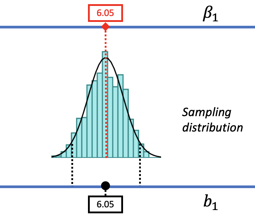
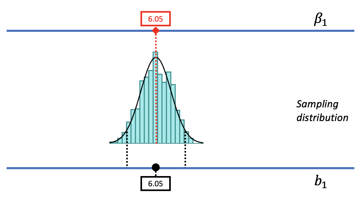
We can start by positioning the DGP and its sampling distribution centered at the sample \(b_1\) of $6.05. It makes sense to start here because \(b_1\) is the best point estimate of the DGP, and it is an unbiased estimator, meaning that the true \(\beta_1\) could be higher or could be lower, but is just as likely to be higher as it is lower.
In the picture below, we slide the DGP and its sampling distribution down (to the left), until we reach a value of the DGP where the sample \(b_1\) is about to fall into the unlikely tail. When we get down to a \(\beta_1\) of -$0.67, we can see that the sample \(b_1\) falls right at the boundary of what we would call unlikely. Thus, -$0.67 is the value of \(\beta_1\) that marks the lower bound of the 95% confidence interval.
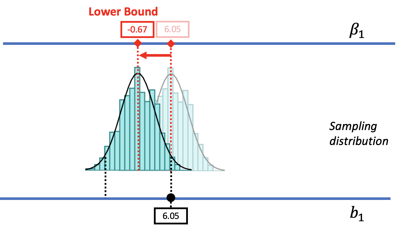
If we were to move the \(\beta_1\) lower than -0.67, the sampling distribution would also move further down and the observed \(b_1\) would become less and less likely to have been generated from these lower DGPs. In this way, we have found a lower bound for the 95% confidence interval: there is a less than .025 chance for any value of \(\beta_1\) lower than -$0.67 to have generated a sample \(b_1\) of $6.05.
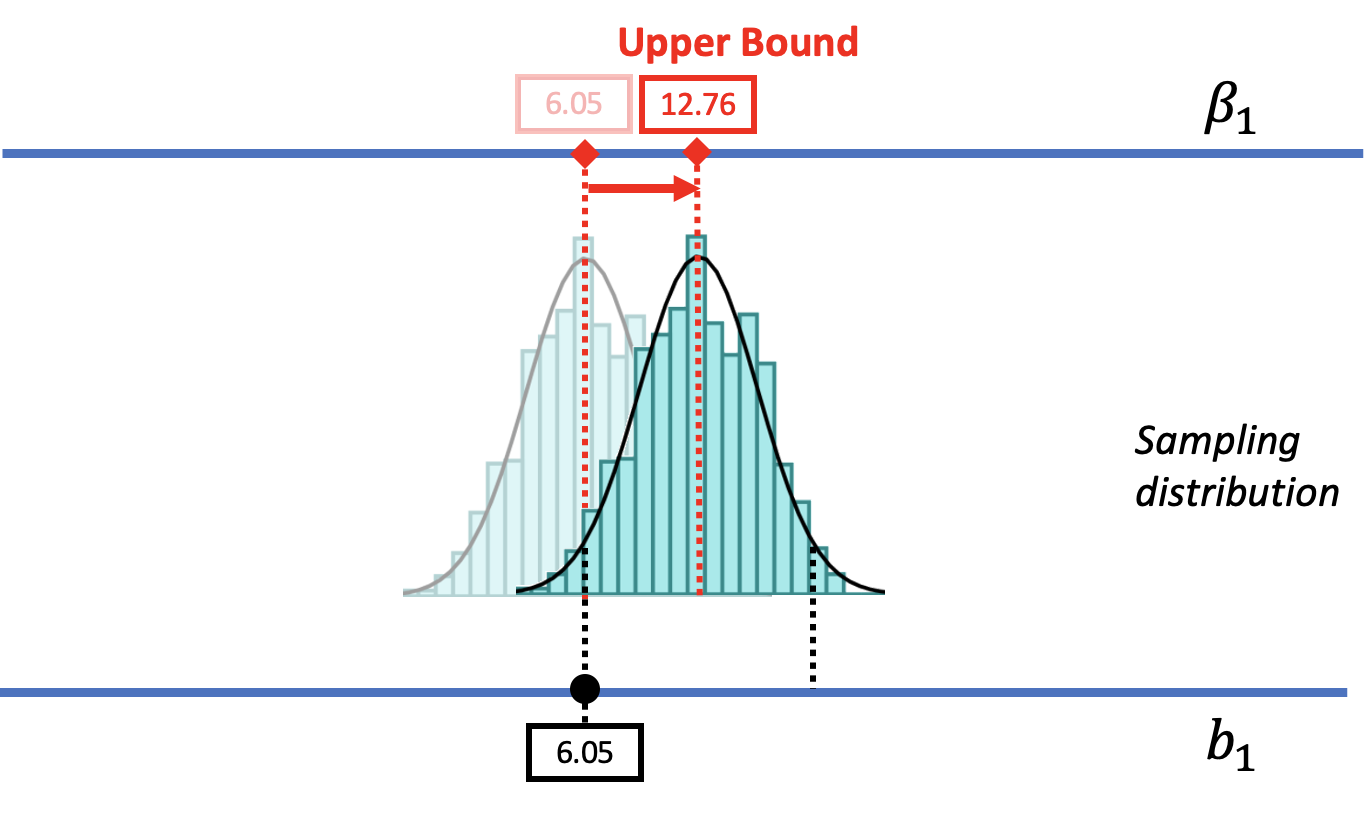
We can use a similar approach to find the upper bound of the confidence interval. As we move the DGP up (to the right), we can consider larger possible values of \(\beta_1\). At some point, as we move the sampling distribution up, we will see the sample \(b_1\) fall into the lower tail of the sampling distribution. When we get to a \(\beta_1\) of 12.76, the \(b_1\) of $6.05 falls past the cutoff into the region we would call unlikely. This value of \(\beta_1\) is considered the upper bound of the 95% confidence interval.
The lower bound and upper bound of a confidence interval indicate the range of \(\beta_1\)s that we would consider likely to have produced the sample \(b_1\).
Putting it all together, we can illustrate the 95% confidence interval, and how it relates to the sampling distribution of \(b_1\), like this:
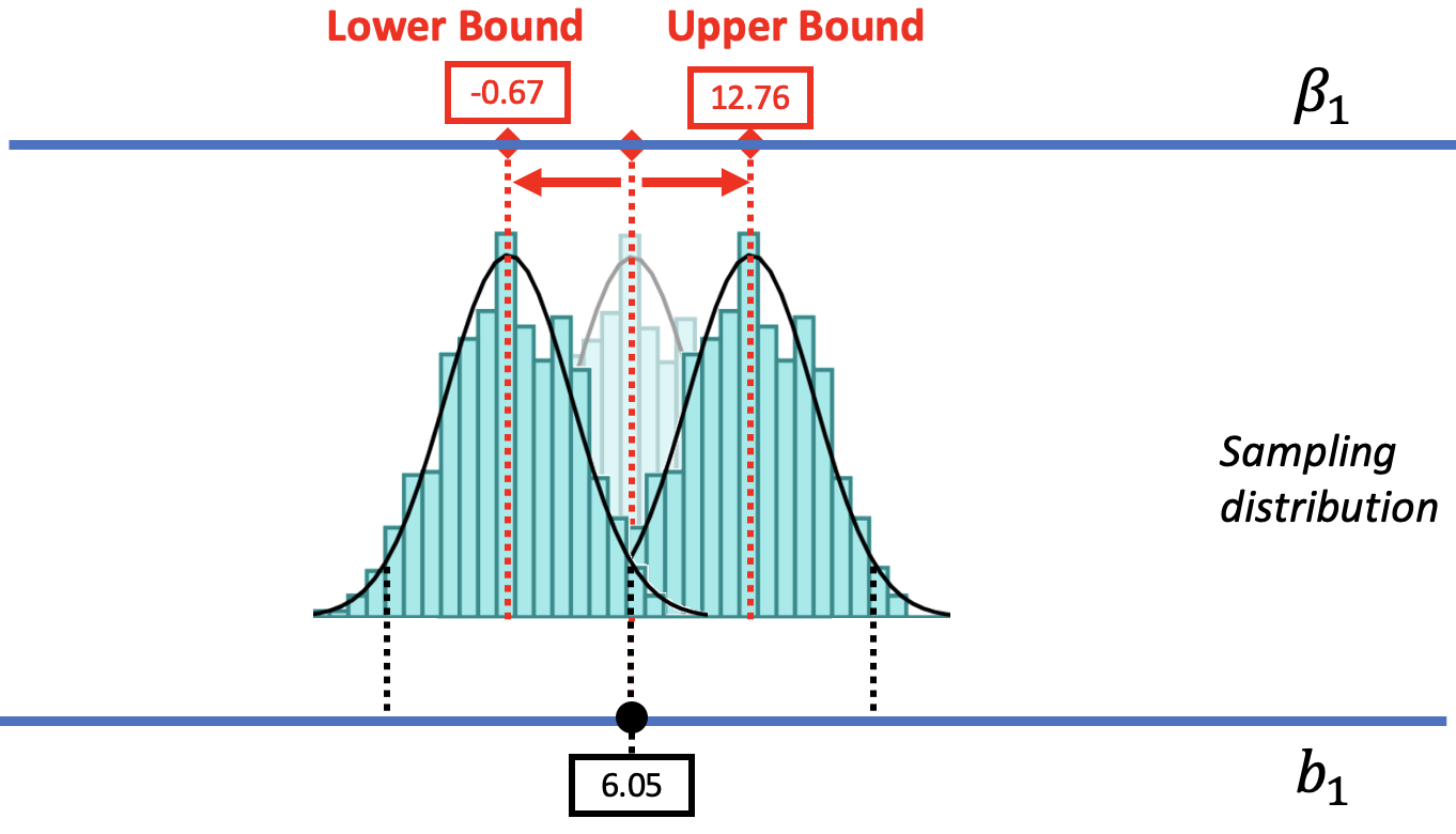
If the sample \(b_1\) has only a .025 chance of being from a DGP lower than the lower bound, and a .025 chance of being from a DGP higher than the upper bound, it follows that we can be 95% confident that the true \(\beta_1\) is somewhere between the two boundaries. This interval is the 95% confidence interval.