7.7 Comparing Two Models: Proportional Reduction in Error
DATA = MODEL + ERROR
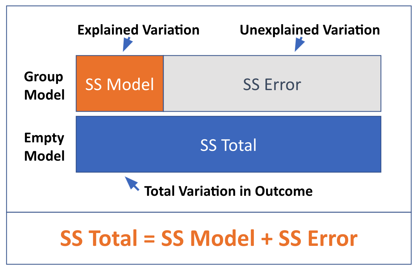
Statistical modeling is all about explaining variation. SS Total tells us how much total variation there is to be explained. When we fit a model (as we have done with the Sex model), that model explains some of the total variation, and leaves some of that variation still unexplained.
These relationships are visualized in the diagram below: Total SS can be seen as the sum of the Model SS (the amount of variation explained by a more complex model) and SS Error, which is the amount left unexplained after fitting the model. Just as DATA = MODEL + ERROR, SS Total = SS Model + SS Error.
Partitioning Sums of Squares
Let’s see how this concept works in the ANOVA table for the Tiny_Sex_model (reprinted below). Look just at the column labeled SS (highlighted). If it looks like an addition problem to you, you are right. The two rows associated with the Sex model (Model and Error) add up to the Total SS (the empty model). So, 54 + 28 = 82.
Analysis of Variance Table (Type III SS)
Model: Thumb ~ Sex

                            SS df     MS     F    PRE     p
----- --------------- | ------  - ------ ----- ------ -----
Model (error reduced) | 54.000  1 54.000 7.714 0.6585 .0499
Error (from model)    | 28.000  4  7.000
----- --------------- | ------  - ------ ----- ------ -----
Total (empty model)   | 82.000  5 16.400
We revised the diagram to more accurately represent the sums of squares in this ANOVA table.
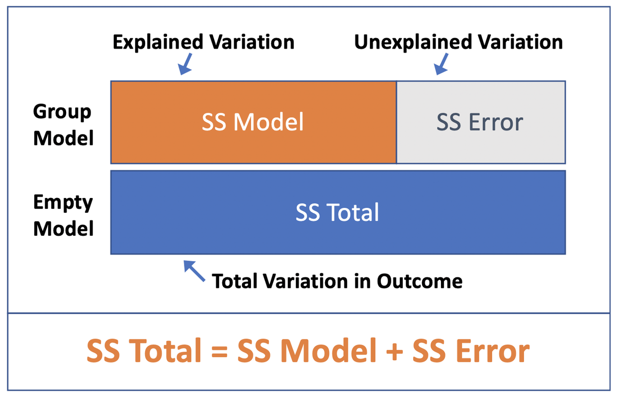
In the diagram, the blue bar represents SS Total, or the total amount of variation in the outcome variable. SS Total, recall, is the sum of the squared distances of each score from the empty model prediction (i.e., the mean). (We saved these distances earlier in a variable called empty_resid.)
The orange and grey bars show how this total variation is partitioned into two parts: the part explained by the Sex model (orange bar), and the part left unexplained by the Sex model (grey bar).
We calculate SS Error (the grey bar) in much the same way we calculate SS Total, except this time we start with residuals from the Sex model predictions instead of from the empty model. (We saved these residuals earlier in a variable called Sex_resid.)
Specifically, we take each score and subtract its predicted value under the Sex model (which is its group mean, be it male or female), square the result, and then add up the squared residuals to get SS Error. SS Error is the amount of variation, measured in sum of squares, that is left unexplained by the Sex model.
The orange bar (SS Model, which is 54 for the Sex model) represents the part of SS Total that is explained by the Sex model. Another way to think of it is as the reduction in error (measured in sums of squares) achieved by the Sex model as compared to the empty model.
There are two ways to calculate SS Model. One is to simply subtract the SS Error (error from the Sex model predictions) from SS Total (error around the mean, or the empty model). Thus:
\[S\!S_{MODEL} = S\!S_{TOTAL} - S\!S_{ERROR}\]
To more directly calculate SS Model, we need to figure out how much error has been reduced by the Sex model in comparison to the empty model. This reduction in error is calculated by taking the distance from each person’s predicted score under the Sex_model to their predicted score under the empty model, squaring it, and then totaling up the squares to get SS Model.
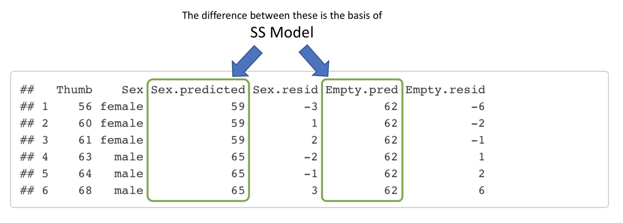
You can think of SS Total = SS Model + SS Error in this more detailed way:
SS(Thumb to empty_model) = SS(Sex_model to empty_model) + SS(Thumb to Sex_model)
The supernova() function tell you that SS Model for the Sex model in the TinyFingers data set is 54. But let’s use R to calculate it step by step, just to see if we get the same result, and also to make sure you understand what’s going on in the supernova() calculation.
Let’s start by adding a new variable called error_reduced in TinyFingers.
TinyFingers$error_reduced <- TinyFingers$Sex_predicted - TinyFingers$empty_predTo calculate the sum of squares for error reduced, we square each person’s value for error_reduced, and sum these squares up across people.
sum(TinyFingers$error_reduced^2)Try this yourself in the code window below to see if you get 54 (the SS Model reported in the supernova table).
require(coursekata)

TinyFingers <- data.frame(
    Sex = as.factor(rep(c("female", "male"), each = 3)),
    Thumb = c(56, 60, 61, 63, 64, 68)
)
Tiny_empty_model <- lm(Thumb ~ NULL, data = TinyFingers)
Tiny_Sex_model <- lm(Thumb ~ Sex, data = TinyFingers)

TinyFingers <- TinyFingers %>% mutate(
    Sex_predicted = predict(Tiny_Sex_model),
    Sex_resid = Thumb - Sex_predicted,
    Sex_resid2 = resid(Tiny_Sex_model),
    empty_pred = predict(Tiny_empty_model)
)
# this creates a column for error reduced by the Sex_model
TinyFingers$error_reduced <- TinyFingers$Sex_predicted - TinyFingers$empty_pred

# add code to sum up the squared error_reduced
TinyFingers$error_reduced <- TinyFingers$Sex_predicted - TinyFingers$empty_pred
sum(TinyFingers$error_reduced^2)
ex() %>% {
    check_object(., "TinyFingers") %>% check_equal()
    check_function(., "sum") %>% check_result() %>% check_equal()
}[1] 54Proportional Reduction in Error (PRE)
We have now quantified how much variation has been explained by our model: 54 square millimeters. Is that good? Is that a lot of explained variation? It would be easier to understand if we knew the proportion of total error that has been reduced rather than the raw amount of error reduced measured in \(mm^2\).
If you take another look at the supernova() table (reproduced below) for the Tiny_Sex_model, you will see a column labelled PRE. PRE stands for Proportional Reduction in Error.
Analysis of Variance Table (Type III SS)
Model: Thumb ~ Sex

                            SS df     MS     F    PRE     p
----- --------------- | ------  - ------ ----- ------ -----
Model (error reduced) | 54.000  1 54.000 7.714 0.6585 .0499
Error (from model)    | 28.000  4  7.000
----- --------------- | ------  - ------ ----- ------ -----
Total (empty model)   | 82.000  5 16.400
PRE is calculated using the sums of squares. It is simply SS Model (i.e., the sum of squares reduced by the model) divided by SS Total (or, the total sum of squares in the outcome variable under the empty model). We can represent this in a formula:
\[P\!R\!E=\frac{S\!S_{Model}}{S\!S_{Total}}\]
In this course, we always will calculate PRE this way, dividing SS Model by SS Total. Based on this formula, PRE can be interpreted as the proportion of total variation in the outcome variable that is explained by the explanatory variable. It tells us something about the overall strength of our statistical model. For example, in our tiny data set (TinyFingers), the effect of Sex on Thumb is fairly strong, with variation in sex accounting for .66 of the variation in thumb length.
It is important to remember that SS Model in the numerator of the formula above represents the reduction in error when going from the empty model to the more complex model, which includes an explanatory variable. To make this clearer we can re-write the above formula like this:
\[P\!R\!E=\frac{S\!S_{Total}-S\!S_{Error}}{S\!S_{Total}}\]
The numerator of this formula starts with the error from the simple (empty) model (SS Total), and then subtracts the error from the complex model (SS Error) to get the error reduced by the complex model. Dividing this reduction in error by the SS Total yields the proportion of total error in the empty model that has been reduced by the complex model.
Although in the current course we always use PRE to compare a complex model to the empty model, the comparison doesn’t need to be to the empty model. In fact, PRE can be used to compare any two models of an outcome variable as long as one is simpler than the other.
It’s good to start thinking now about how to use PRE for comparing more complicated models to each other. Toward this end, we will add one more version of the same formula that is easier to apply to all model comparisons in the future:
\[P\!R\!E=\frac{S\!S_{Error\>from\>Simple\>Model}-S\!S_{Error\>from\>Complex\>Model}}{S\!S_{Error\>from\>Simple\>Model}}\]
Just as a note: when, as in the current course, PRE is used to compare a complex model to the empty model, it goes by other names as well. In the ANOVA tradition (Analysis of Variance) it is referred to as \(\eta^2\), or eta squared. In Chapter 8 we will introduce the same concept in the context of regression, where it is called \(R^2\). For now all you need to know is: these are different terms used to refer to the same thing, in case anyone asks you.
Fitting the Sex Model to the Full Fingers Data Set
Before moving on, use the code window below to fit the Sex model to the full Fingers data set. Save the model in an R object called Sex_model. Print out the model (this will show you the values of \(b_{0}\) and \(b_{1}\)). Then run supernova() to produce the ANOVA table.
require(coursekata)
# fit the model Thumb ~ Sex with the Fingers data
# save it to Sex_model
Sex_model <- lm(formula = , data = )

# print out the model


# print the supernova table for Sex_model
# fit the model Thumb ~ Sex with the Fingers data
# save it to Sex_model
Sex_model <- lm(formula = Thumb ~ Sex, data = Fingers)

# print out the model
Sex_model

# print the supernova table for Sex_model
supernova(Sex_model)
ex() %>% {
    check_object(., "Sex_model") %>% check_equal()
    check_output_expr(., "Sex_model")
    check_output_expr(., "supernova(Sex_model)")
}Call:
lm(formula = Thumb ~ Sex, data = Fingers)
Coefficients:
(Intercept) Sexmale
58.256 6.447Analysis of Variance Table
Outcome variable: Thumb
Model: lm(formula = Thumb ~ Sex, data = Fingers)
SS df MS F PRE p
----- ----------------- --------- --- -------- ------ ------ -----
Model (error reduced) | 1334.203 1 1334.203 19.609 0.1123 .0000
Error (from model) | 10546.008 155 68.039
----- ----------------- --------- --- -------- ------ ------ -----
Total (empty model) | 11880.211 156 76.155