Chapter 10: Model Comparison with F
10.1 Moving Beyond b1
In the previous chapter we learned how to use the sampling distribution of \(b_1\) to evaluate the empty model. Using the shuffle() function, we generated a sampling distribution for a world in which the empty model is true in the DGP, i.e., \(\beta_1=0\). We used the sampling distribution to calculate the p-value, the probability that the sample \(b_1\), or a \(b_1\) more extreme than the sample, would have occurred just by chance if the empty model were true. Based on the p-value, and the decision criterion we had set (i.e., the alpha of .05), we decided whether to reject the empty model of the DGP or not.
As it turns out, the sampling distribution of \(b_1\) is just one of many sampling distributions we could construct. Using the same approach we developed with \(b_1\), we could make a sampling distribution of \(b_0\), the median, the standard deviation, and more. Any statistic we can calculate from a sample of data would vary with each new sample of data, which is why we can think of any statistic as coming from a sampling distribution.
In this chapter we are going to extend our understanding of randomization beyond the sampling distribution of \(b_1\). We will focus on the sampling distributions of PRE and F. The sampling distribution of F, especially, is widely used for model comparison, and is more generalizable to many situations than is the sampling distribution of \(b_1\).
Reviewing the Concepts of PRE and F
Both PRE and F provide a means of comparing two models: one that includes an explanatory variable (a more complex model) with one that does not (the empty model). Let’s use the tipping experiment, again, to remind us of what PRE and F are and what they mean. Researchers wanted to figure out the effect of smiley faces on tips: Did tables randomly assigned to get smiley faces on their checks give higher tips than tables that got no smiley faces?
We can restate this question as a comparison between two models of the data: the empty model, in which the grand mean is used to predict tips; and the best-fitting two-group model, in which the group means for the smiley and no smiley conditions are used to predict tips.
These two models of the data can be represented in GLM notation like this:
\(Y_i = b_0 + b_1X_i + e_i\) (the two-group model); and
\(Y_i = b_0 + e_i\) (the empty model)
Note that the two-group model, in this case, could be referred to as the “complex model,” the empty model as the “simple model.” Complex and simple are relative terms. When we compare two models, one is generally more complex than the other; but the simple model does not always have to be the empty model (though in this case it is).
The PRE, or Proportional Reduction in Error, is the proportion of total variation in the outcome variable that is explained by using the more complex model over the simple one. Another way of saying this is that PRE is the proportion of Sum of Squares Total that is reduced by the complex model over the empty model. (This is just a recap of what you learned in prior chapters.)
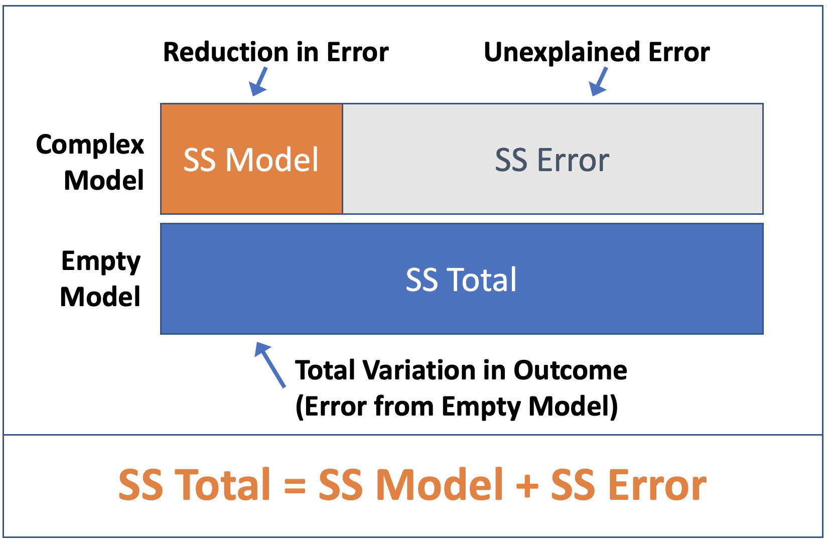
The F ratio is the ratio of two variances (or Mean Squares): MS Model divided by MS Error. F is closely related to PRE but it takes into account the number of degrees of freedom used to fit the complex model. Both PRE and F are ways of quantifying the strength of the relationship between the explanatory and outcome variables. You can think of F as a measure of the strength of a relationship (like PRE) per parameter included in the model.
Although in general, more complex models explain more error (i.e., have greater PRE), F balances the desire to explain variation against using degrees of freedom foolishly. Thus, F gives us a reasonable way to compare models that use a lot of parameters (e.g., \(Y_i = b_0 + b_1X_{1i} + b_2X_{2i} + b_3X_{3i}...\)) against the empty model that only uses 1.
We can get both the PRE and F from the ANOVA table that is generated by the supernova() function. Use the code window below to fit the Condition_model to the tipping experiment data, and then generate the ANOVA table.
require(coursekata)
# this saves the best fitting complex model in Condition_model
            Condition_model <- lm(Tip ~ Condition, data = TipExperiment)

            # generate the ANOVA table for the complex model
# this saves the best fitting complex model in Condition_model
Condition_model <- lm(Tip ~ Condition, data=TipExperiment)

# generate the ANOVA table for the complex model
supernova(Condition_model)
# Or
supernova(lm(Tip ~ Condition, data = TipExperiment))
ex() %>% {
       check_function(., "supernova") %>%
       check_result() %>%
       check_equal()
}Analysis of Variance Table (Type III SS)
Model: Tip ~ Condition
SS df MS F PRE p
----- ----------------- -------- -- ------- ----- ------ -----
Model (error reduced) | 402.023 1 402.023 3.305 0.0729 .0762
Error (from model) | 5108.955 42 121.642
----- ----------------- -------- -- ------- ----- ------ -----
Total (empty model) | 5510.977 43 128.162 We can see from the ANOVA table that adding Condition to the model results in a PRE of .07. This means that .07 of the error from the empty model is reduced, or explained, by the complex model.
That the PRE is greater than 0 is no surprise, however. The only way PRE would be equal to 0 is if there were no mean difference at all between the two groups in the sample (that is, if \(b_1 = 0\)). In that case, knowing which group a table was in (Smiley Face or Control) would add no predictive value, and thus result in 0 reduction in error.
But even if there were no effect of smiley face in the DGP, we would rarely get a sample with no mean difference at all between the groups. Because of random sampling variation, even when two groups are generated by the same DGP from the same population, it would be rare to get two identical means (e.g., a mean difference of 0).