7.5 Examining Residuals From the Model
As we have said before, when we use a model to make predictions, our predictions are usually wrong. The residuals, or the distance of each observed score from the predicted score, give us an indication of how wrong our predictions are for each person.
Calculating Residuals From the Model
We calculated residuals from the empty model by subtracting the mean from each score. We use the same approach for the more complex model.
Using the model, we assign a predicted score to each observation. This time, however, the predicted score is not the Grand Mean for everyone, but one mean for females and another for males.
Notice that we use the same strategy to quantify the leftover error from any model. We can do the subtractions in R, just as we did for the empty model. We start with the TinyFingers data frame looking like this.
     Sex Thumb Sex_predicted
1 female    56            59
2 female    60            59
3 female    61            59
4   male    63            65
5   male    64            65
6   male    68            65
We then calculate the residual for each person by this subtraction: their observed score minus their score predicted by the model. We will save the result in a new variable in TinyFingers that we will call Sex_resid.
TinyFingers$Sex_resid <- TinyFingers$Thumb - TinyFingers$Sex_predicted
TinyFingers
Sex Thumb Sex_predicted Sex_resid
1 female 56 59 -3
2 female 60 59 1
3 female 61 59 2
4 male 63 65 -2
5 male 64 65 -1
6 male 68 65 3Another, slightly easier, way to do the same thing is to use the resid() function, using the Tiny_Sex_model as the argument. Let’s try that, and save the results in a new variable, Sex_resid2. Then let’s print the updated version of TinyFingers.
TinyFingers$Sex_resid2 <- resid(Tiny_Sex_model)
TinyFingers
Sex Thumb Sex_predicted Sex_resid Sex_resid2
1 female 56 59 -3 -3
2 female 60 59 1 1
3 female 61 59 2 2
4 male 63 65 -2 -2
5 male 64 65 -1 -1
6 male 68 65 3 3 Compare the two variables—Sex_resid and Sex_resid2—in the output. Notice that we get the same values for Sex_resid2 as we did for Sex_resid.
Finally, let’s compare the residuals from the Tiny_Sex_model to those from the Tiny_empty_model. Let’s first add a variable called empty_pred using the predict() function, and print out TinyFingers again. (We could have called the variable anything; the point is to name it something meaningful—so in this case we called it empty_pred, short for predicted from the empty model.)
TinyFingers$empty_pred <- predict(Tiny_empty_model)
TinyFingers
Sex Thumb Sex_predicted Sex_resid Sex_resid2 empty_pred
1 female 56 59 -3 -3 62
2 female 60 59 1 1 62
3 female 61 59 2 2 62
4 male 63 65 -2 -2 62
5 male 64 65 -1 -1 62
6 male 68 65 3 3 62 Now use the resid() function to create a new variable in the TinyFingers data frame, empty_resid. And print out the updated version of TinyFingers.
require(coursekata)

TinyFingers <- data.frame(
    Sex = as.factor(rep(c("female", "male"), each = 3)),
    Thumb = c(56, 60, 61, 63, 64, 68)
)
Tiny_empty_model <- lm(Thumb ~ NULL, data = TinyFingers)
Tiny_Sex_model <- lm(Thumb ~ Sex, data = TinyFingers)

TinyFingers <- TinyFingers %>% mutate(
    Sex_predicted = predict(Tiny_Sex_model),
    Sex_resid = Thumb - Sex_predicted,
    Sex_resid2 = resid(Tiny_Sex_model),
    empty_pred = predict(Tiny_empty_model)
)
# generate residuals from Tiny_empty_model
 TinyFingers$empty_resid <-

# write code to print TinyFingers
TinyFingers$empty_resid <- resid(Tiny_empty_model)
TinyFingers
ex() %>% {
    check_object(., "TinyFingers")
    check_output_expr(., "print(TinyFingers)")
} Sex Thumb Sex_predicted Sex_resid Sex_resid2 empty_pred empty_resid
1 female 56 59 -3 -3 62 -6
2 female 60 59 1 1 62 -2
3 female 61 59 2 2 62 -1
4 male 63 65 -2 -2 62 1
5 male 64 65 -1 -1 62 2
6 male 68 65 3 3 62 6Graphing Residuals From the Model
You might wonder, why are we bothering to generate and save residuals? We will have a lot more to say about this later. But the short answer is: it helps us to understand the error around our model, and often suggests ways of improving the model.
Just as the first thing we do when looking at a data set is to examine the distributions of the variables, it is good to get in the habit of examining the distributions of residuals after we fit a new model.
Let’s go back to the full Fingers data frame. We fit the model lm(Thumb ~ Sex, data = Fingers) and saved the model in Sex_model. Using the resid() function, write some code to generate a new column in Fingers called Sex_resid (the residuals from the Sex_model).
require(coursekata)

Sex_model <- lm(Fingers$Thumb ~ Fingers$Sex)
# store the residuals from Sex_model
Fingers$Sex_resid <-

# This prints the first 10 rows of Fingers
head(select(Fingers, Thumb, Sex_resid), 10)
# store the residuals from Sex_model
Fingers$Sex_resid <- resid(Sex_model)

# This prints the first 10 rows of Fingers
head(select(Fingers, Thumb, Sex_resid), 10)
ex() %>% {
  check_object(., "Fingers") %>%
    check_column("Sex_resid") %>%
    check_equal()
}In the following window, we have provided the code to create density histograms of Thumb in a facet grid by Sex. Try modifying it to generate density histograms of Sex_resid in a facet grid by Sex. Compare the histograms of residuals from the Sex_model with histograms of thumb length.
require(coursekata)

Sex_model <- lm(Fingers$Thumb ~ Fingers$Sex)
Fingers$Sex_resid <- resid(Sex_model)
# This creates histograms of Thumb for each Sex
# Modify it to create histograms of Sex_resid for each Sex
gf_dhistogram(~Thumb, data = Fingers) %>%
    gf_facet_grid(Sex ~ .)
# This creates histograms of Thumb for each Sex
# Modify it to create histograms of Sex_resid for each Sex
gf_dhistogram(~Sex_resid, data = Fingers) %>%
    gf_facet_grid(Sex ~ .)
ex() %>% {
    check_or(.,
        check_function(., "gf_dhistogram") %>% {
            check_arg(., "object") %>% check_equal()
            check_arg(., "data") %>% check_equal()
        },
        override_solution(., "gf_dhistogram(Fingers, ~Sex_resid)") %>%
            check_function("gf_dhistogram") %>% {
            check_arg(., "object") %>% check_equal()
            check_arg(., "gformula") %>% check_equal()
        }
    )
    check_function(., "gf_facet_grid") %>%
        check_arg("...") %>%
        check_equal(incorrect_msg = "Make sure you keep the code to create a grid faceted by `Sex`")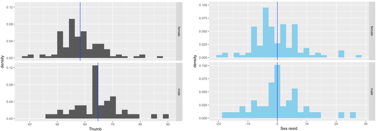
}In the activity below, we’ve depicted the density histograms of Thumb by Sex (in black) next to the histograms of Sex_resid by Sex (in skyblue).
We can add the means of Thumb for females and males to the Thumb histograms with some R code. First, we calculate the mean Thumb length for each Sex group and save it in an R object called Thumb_stats:
Thumb_stats <- favstats(Thumb ~ Sex, data = Fingers)Then we chain on (%>%) a vertical line on our histogram with this code.
gf_vline(xintercept = ~mean, data = Thumb_stats)Here we have provided the code to add mean lines for each Sex group to the Thumb histograms. Modify the next chunk of code to add mean lines for each Sex group to the Sex_resid histograms.
require(coursekata)

Sex_model <- lm(Fingers$Thumb ~ Fingers$Sex)
Fingers$Sex_resid <- resid(Sex_model)
# this creates histograms with lines at the mean of Thumb length for each Sex
Thumb_stats <- favstats(Thumb ~ Sex, data = Fingers)
gf_dhistogram(~Thumb, data = Fingers) %>%
    gf_facet_grid(Sex ~ .) %>%
    gf_vline(xintercept = ~mean, color = "blue", data = Thumb_stats)

# modify this code to add lines to represent the mean Sex_resid of each Sex group
Sex_resid_stats <- favstats(Sex_resid ~ Sex, data = Fingers)
gf_dhistogram(~Sex_resid, data = Fingers, fill = "skyblue") %>%
    gf_facet_grid(Sex ~ . )
Thumb_stats <- favstats(Thumb ~ Sex, data = Fingers)
    gf_dhistogram( ~ Thumb, data = Fingers) %>%
     gf_facet_grid(Sex ~ .) %>%
     gf_vline(xintercept = ~mean, color = "blue", data = Thumb_stats)

Sex_resid_stats <- favstats(Sex_resid ~ Sex, data = Fingers)
gf_dhistogram( ~ Sex_resid, data = Fingers, fill = "skyblue") %>%
    gf_facet_grid(Sex ~ . ) %>%
    gf_vline(xintercept = ~mean, color = "blue", data = Sex_resid_stats)
ex() %>% {
    check_function(., "gf_vline", index = 1)
    check_function(., "gf_vline", index = 2)
    check_function(., "gf_facet_grid", index = 1)
    check_function(., "gf_facet_grid", index = 2)
    check_function(., "gf_dhistogram", index = 1)
    check_function(., "gf_dhistogram", index = 2) %>%
        check_arg("data") %>% check_equal()
}