Chapter 8 - Models With a Quantitative Explanatory Variable
In the previous chapter we figured out how to add an explanatory variable to a model. We explained thumb length using sex, and using height (coded as short/tall, or short/medium/tall). We noticed two things: First, when we add more groups, we reduce left over error, explaining more variation in our outcome variable.
But, second, when we add more groups we use more degrees of freedom. If we keep going like this, we certainly will explain lots of variation in our data, but our explanation will not be very elegant. Imagine if we had a “group” for every individual in our sample. We would explain all the variability, but have a completely useless model in terms of understanding the Data Generating Process (DGP).
Let’s consider another approach: instead of using height in inches to divide students into groups (e.g., short or tall), what if we just model height as a continuous variable? Earlier in the course we learned how to visualize this approach in a scatterplot. In this chapter we will figure out how to extend our models to accommodate quantitative explanatory variables.
The models we develop in this chapter are usually called regression models. Before we start, though, note that the core ideas behind these new models are exactly the same as those we have developed for the grouping models. A model still yields a single predicted score for each observation, based on some mathematical function of the explanatory variable.
Further, in regression models, we still use residuals—the difference between the predicted and observed score to measure error around the model; and we still use the sum of squared deviations from the model predictions as a measure of model fit. And, we still use PRE to indicate the proportion reduction in error of the regression model compared with the empty model.
8.1 Groups versus Quantitative Explanatory Variables
The Two-Group Model: Review
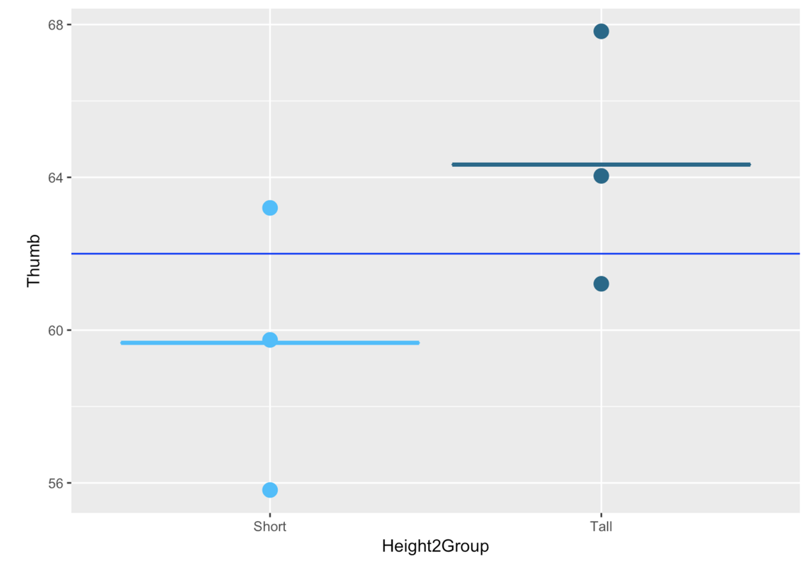
Let’s start with our TinyFingers data set. In the graph below, we illustrate the two-group approach to modeling this data. Just as a reminder, we would specify this model—the Height2Group model—as a two-parameter model, with one parameter being the mean thumb length for short people, the other, the increment to add on for tall people.
We can represent this two-group model like this:
\[Y_{i}=b_{0}+b_{1}X_{i}+e_{i}\]
Or like this:
\[{Thumb}_{i}=b_{0}+b_{1}{Height2Group}_{i}+e_{i}\]
Although \(X_{i}\) is coded this way by R, you could, in theory, code it different ways. R has coded the first group (in this case, the short group) as 0 and the next group (the tall group) as 1. Doing this makes the interpretation of \(b_{1}\) straightforward: it is the estimated increment in thumb size from short people to tall people.
Note that the increment to add on for short people would be negative: by starting with \(b_{0}\) as the mean for tall people, \(b_{1}\) would represent the decrement when going from the mean for tall people to the mean for short people.
In general, the reason we code 0 for short and 1 for tall in this situation is simply that it makes the interpretation easier to keep in our brains! It’s easier to think of an increment than a decrement, for some reason. If we did decide to switch the coding, though, we would probably want to reverse the order in the graph to make the graph more consistent with the model.
We are comparing the Height2Group model to the empty model, which is represented in the graph above with the blue horizontal line that goes all the way across the plot. The predicted score for everyone under the empty model is the Grand Mean.
The SS Total for the Height2Group model is the sum of squared deviations from the empty model. The SS Error for the Height2Group model is the deviation of each score from its group mean (Short or Tall).
We can see just by inspecting the graph above that the two-group model will yield better predictions than the empty model. Knowing whether someone is short or tall would help us make a more accurate prediction of their thumb length than if we didn’t know which group they were in (in which case we would just use the empty model).
The Continuous Model
Now let’s compare what happens when we use Height as a quantitative variable instead of as a grouping variable.
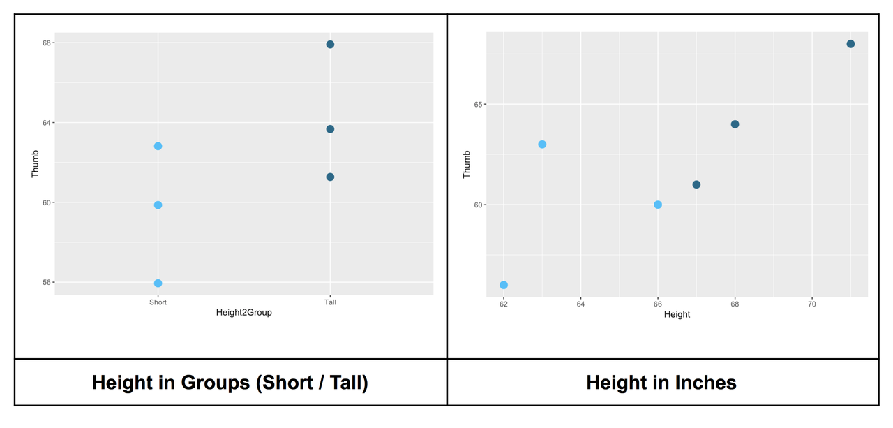
The scatterplot below (right) shows Height on the x-axis measured in inches (the explanatory variable) and thumb length measured in millimeters on the y-axis (the outcome variable). We have included the Height2Group plot on the left, for comparison.
The same six data points are represented in the graph on the left (which uses Height2Group as the explanatory variable) as in the graph on the right, (which uses Height in inches). Whereas the points on the left are divided into two groups, the points on the right are spread out continuously over the x-axis, with each person’s height and thumb length represented as a point in two-dimensional space.
The empty model can be represented the same way in both graphs, by a horizontal line through the Grand Mean.
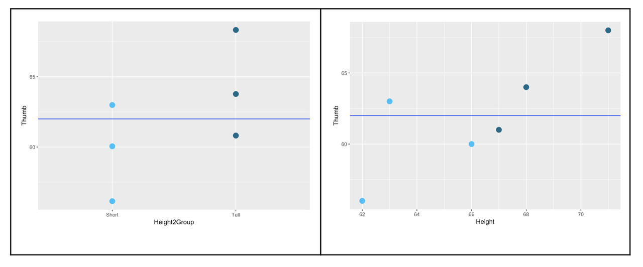
The empty model of the outcome variable is exactly the same no matter how you code the explanatory variable: it is just the mean of the six data points. Sum of squared deviations around the empty model, thus, is the same in both cases.
We get a sense from the scatterplot that knowing someone’s exact height would help us make a better prediction of their thumb length than just knowing whether they are short or tall. But where, in the scatterplot, is the model?
When the explanatory variable is categorical, as with Height2Group, we can use the group means as our model (as reviewed above). But when the explanatory variable is quantitative, as with Height in inches, we can’t use the group means to predict new scores because there are no groups!