5.3 The Mean as a Model
Having developed the idea that a single number can serve as a statistical model for a distribution, we now ask: which single number should we choose? We have been talking informally about choosing a number in the middle of a symmetric, normal-shaped distribution. But now we want to get more specific.
Recall that in the previous section we defined a statistical model as a function that produces a predicted score for each observation. Armed with this definition, we can now ask: what function could we use that would generate the same predicted value for all observations in a distribution?
Median and Mean: Two Possible Functions for Generating Model Predictions
If we were trying to pick a number to model the distribution of a categorical variable, we should pick the mode; really, there isn’t much choice here. If you are going to predict the value of a new observation on a categorical variable, the prediction will have to be one of the categories and you will be wrong least often if you pick the most frequently observed category.
For a quantitative variable, statisticians typically choose one of two numbers: the median or the mean. The median is just the middle number of a distribution. Take the following distribution of five numbers:
5, 5, 5, 10, 20
The median is 5, meaning that if you sort all the numbers in order, the number in the middle is 5. You can see that the median is not affected by outliers. So, if you changed the 20 in this distribution to 20,000, the median would still be 5.
To calculate the mean of this distribution, we simply add up all the numbers in the sample, and then divide by the sample size, which is 5. So, the mean of this distribution is 9. Both mean and median are indicators of where the middle of the distribution is, but they define “middle” in different ways: 5 and 9 represent very different points in this distribution.
In R, these and other statistics are very easy to find with the function favstats(). Create a variable called outcome and put in these numbers: 5, 5, 5, 10, 20. Then, run the favstats() function on the variable outcome.
require(coursekata)
# Modify this line to save the numbers to outcome
outcome <- c()

# This will give you the favstats for outcome
favstats(outcome)
outcome <- c(5, 5, 5, 10, 20)
favstats(outcome)
ex() %>% {
    check_object(., "outcome") %>% check_equal()
    check_function(., "favstats") %>% check_result() %>% check_equal()
} min Q1 median Q3 max mean sd n missing
5 5 5 10 20 9 6.519202 5 0If you want, you can save output of favstats() into an R object. Although you can name it whatever you want, it might be helpful to use a rule of thumb like the variable name and the phrase _stats after it.
outcome_stats <- favstats(outcome)When you save the results of favstats(), you end up with a data frame where the columns are the different summary statistics. If you just wanted to output the mean of outcome_stats, you could write outcome_stats$mean. R thinks of mean as a variable in the data frame outcome_stats. R does this because a data frame is a handy way to organize and label a bunch of numbers like our favstats.
If our goal is just to find the single number that best characterizes a distribution, sometimes the median is better, and sometimes the mean is better.
If you are trying to choose one number that would best predict what the next randomly sampled value might be, the median might well be better than the mean for this distribution. With only five numbers, the fact that three of them are 5 leads us to believe that the next one might be 5 as well.
On the other hand, we know nothing about the Data Generating Process (DGP) for these numbers. The fact that there are only five of them indicates that this distribution is probably not a good representation of the underlying population distribution. The population could be normal, or uniform, in which case the mean would be a better model than the median. The point is, we just don’t know.
Realizing this limitation, let’s look at some distributions of quantitative variables, and see which number we think is a summary of each distribution as a whole: median or mean.
For each of these variables, make histograms and get the favstats(). For each distribution, which do you think is a better one-number model? The median or the mean?
require(coursekata)
# modify this code to make a histogram of GradePredict
gf_histogram(~ , data = Fingers)

# get the favstats for GradePredict
gf_histogram(~GradePredict, data = Fingers)
favstats(~GradePredict, data = Fingers)
ex() %>% {
            check_function(., "gf_histogram") %>% check_result() %>% check_equal()
                check_function(., "favstats") %>% check_result() %>% check_equal()
}require(coursekata)
# modify this code to make a histogram of Thumb
gf_histogram()

# get the favstats for Thumb
gf_histogram(~Thumb, data = Fingers)
favstats(~Thumb, data = Fingers)
ex() %>% {
    check_function(., "gf_histogram") %>% check_result() %>% check_equal()
    check_function(., "favstats") %>% check_result() %>% check_equal()
}require(coursekata)
# make a histogram of Age in the MindsetMatters data frame

# get the favstats for Age
gf_histogram(~Age, data = MindsetMatters)
favstats(~Age, data = MindsetMatters)
ex() %>% {
    check_function(., "gf_histogram") %>% check_result() %>% check_equal()
    check_function(., "favstats") %>% check_result() %>% check_equal()
}In general, the median may be a more meaningful summary of a distribution of data than the mean, when the distribution is skewed one way or the other. In essence, this discounts the importance of the tail of the distribution, focusing more on the part of the distribution where most people score. The mean is a good summary when the distribution is more symmetrical.
But, if our goal is to create a statistical model of the population distribution, we almost always—especially in this course—will use the mean. We shall dig in a little to see why. But first, a brief detour to see how we can add the median and mean to a histogram.
Adding Median and Mean to Histograms
You already know the R code to make a histogram.
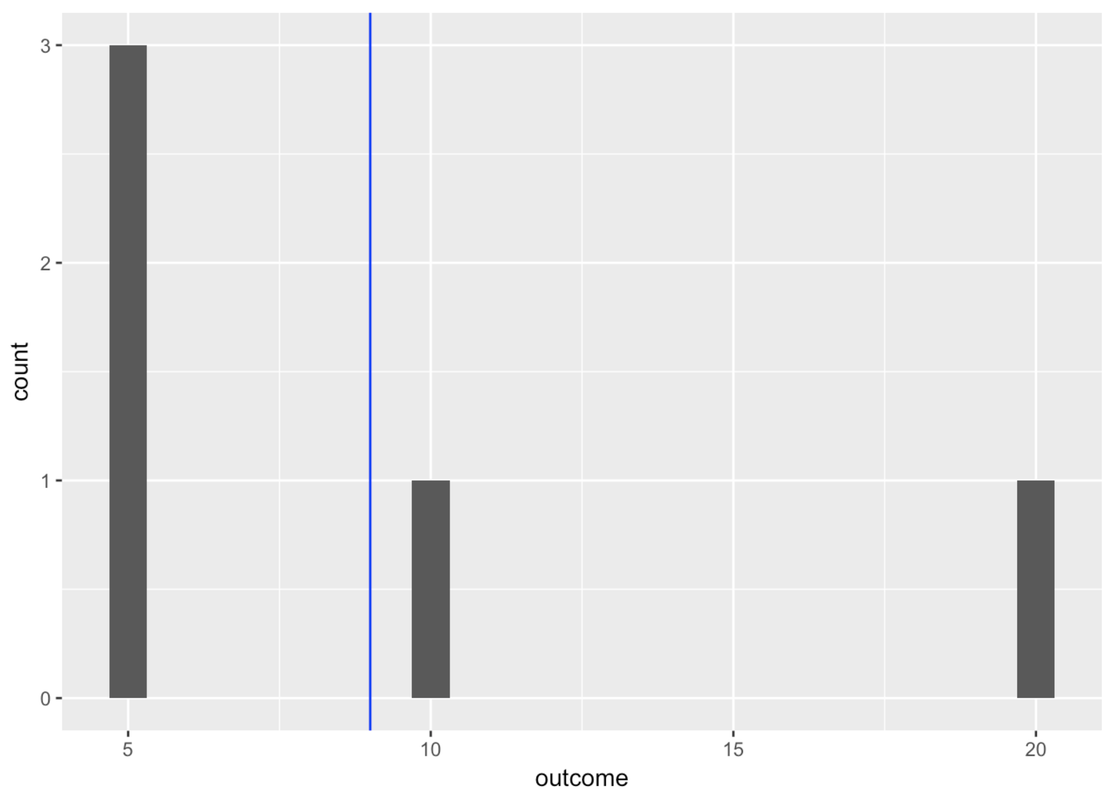
gf_histogram(~ outcome, data = tiny_data)Let’s add a vertical line to show where the mean is. We know from favstats() that the mean is 9, so we can just add a vertical line that crosses the x-axis at 9. Let’s color it blue.
gf_histogram(~ outcome, data = tiny_data) %>%
  gf_vline(xintercept = 9, color = "blue")
Alternatively, if we don’t want to have to remember the mean, we can just take the mean from the output of favstats() we saved earlier.
gf_histogram(~ outcome, data = tiny_data) %>%
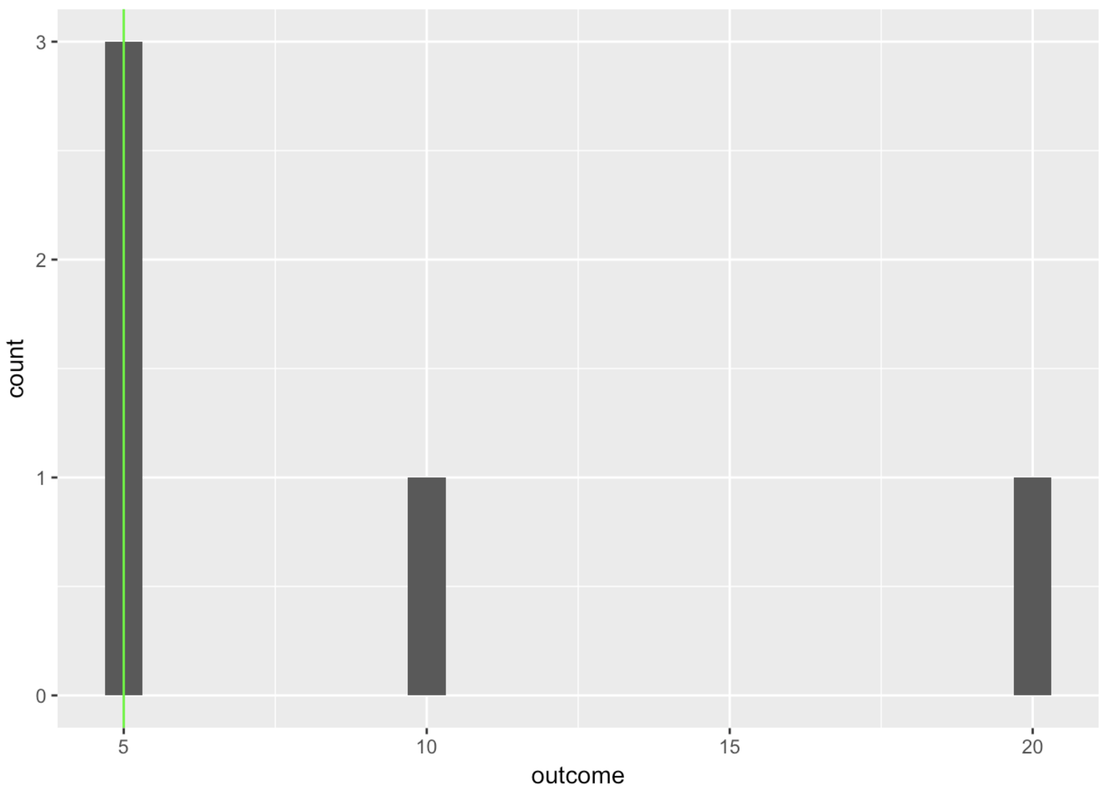
gf_vline(xintercept = ~mean, color = "blue", data = outcome_stats)Try modifying this code to draw a green line for the median using the favstats you’ve saved in outcome_stats.
require(coursekata)

tiny_data <- data.frame(outcome = c(5,5,5,10,20))
outcome_stats <- favstats(~outcome, data = tiny_data)
# We saved the favstats for outcome to outcome_stats
# Modify this to draw a vline representing the median in "green"
gf_histogram(~outcome, data = tiny_data) %>%
  gf_vline(xintercept = ~mean, color = "blue", data = outcome_stats)
gf_histogram(~outcome, data = tiny_data) %>%
  gf_vline(xintercept = ~median, color = "green", data = outcome_stats)
ex() %>% {
    check_function(., "gf_histogram") %>%
        check_result() %>% check_equal()
    check_function(., "gf_vline") %>% {
        check_arg(., "xintercept") %>% check_equal()
        check_arg(., "data") %>% check_equal()
        check_arg(., "color") %>% check_equal()
        check_result(.) %>% check_equal()
    }
}
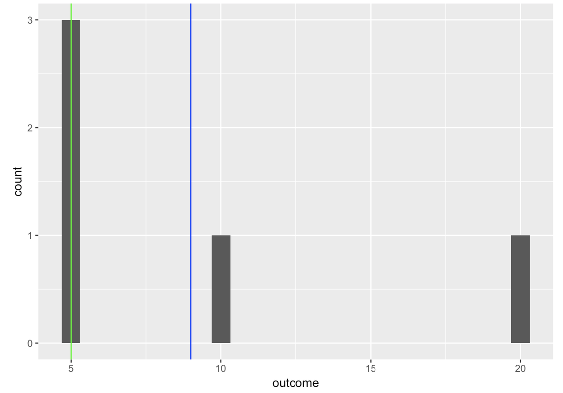
You can string these commands together (using %>%) to put both the mean and median lines onto a histogram.
gf_histogram(~ outcome, data = tiny_data) %>%
  gf_vline(xintercept = ~mean,  color = "blue", data = outcome_stats) %>%
  gf_vline(xintercept = ~median,  color = "green", data = outcome_stats)
Exploring the Mean
It’s pretty easy to understand how the median is the middle of a distribution, but in what sense is the mean the middle? One way to think of the mean is as the balancing point of the distribution, the point at which the things above it equal the things below it. But what does it balance? What are “the things” that are equal on both sides of the mean?
You can either watch the video explanation (with Dr. Ji) or read about it in the section below.
You might think that the values below the mean balance with the values above the mean. Let’s try that. Does 5+5+5 = 10+20? No, 15 does not equal 30. A bunch of smaller values, what we find below the mean, is not going to balance a bunch of larger values (the ones above the mean). So what does the mean balance?
Here it helps to think about each score’s deviation, which is the distance above or below the mean. In our example, each of the 5s are 4 units below the mean of 9, which we will represent as -4. If you think of it this way, the sum of deviations below the mean (-12) balances out the sum of deviations above the mean (+1 and +11, or +12).
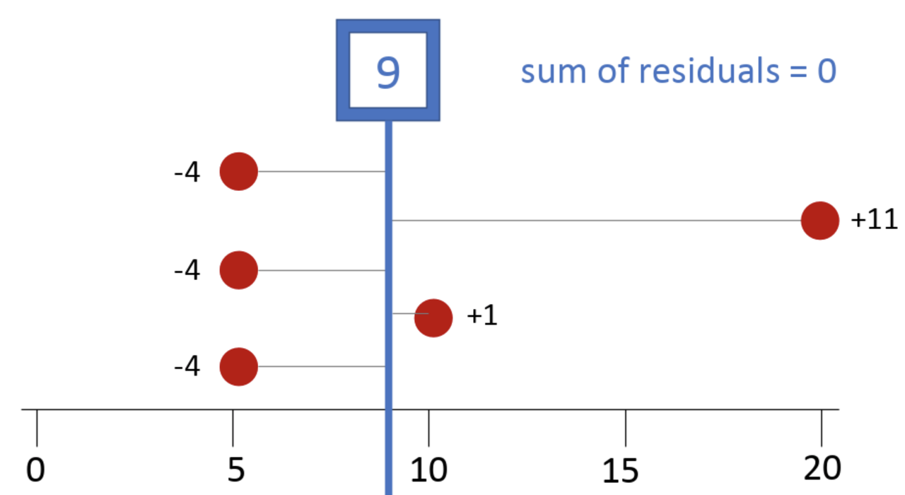
It turns out that no number other than the mean (not 8, not 8.5, not 9.1!) will perfectly balance the deviations above the mean with those below the mean. Whereas the magnitude of a score—especially an outlier—won’t necessarily affect the median, it will affect the mean because the large deviation from an outlier has to be balanced with the deviations from the other data points. Every value gets taken into account when calculating the mean.
Remember we talked about finding some simple shapes that “fit” the more detailed shape of California the best? We wanted to find shapes that were not too big and not too small, shapes that would minimize the error around the model, defined as the parts of California that were not covered by the model, and the parts of the model that covered stuff not in California.
The mean is a model that is not too big and not too small. The mean is pulled in both directions (larger and smaller) at once and settles right in the middle. The mean is the number that balances the amount of deviation above and below it, yielding the same amount of error above it as below it. It’s kind of amazing that this procedure of adding up all the numbers and dividing by the number of numbers results in this balancing point.
Thinking about the mean in this way also helps us think about DATA = MODEL + ERROR in a more specific way. If the mean is the model, each data point can now be thought of as the sum of the model (9 in our tiny_data set) plus its deviation from the model. So 20 can be decomposed into the model part (9) and the error from the model (+11). And 5 can be decomposed into 9 (model) and -4 (error).