2.7 The Structure of Data
Data can come to us in many forms. If you collect data yourself, you may start out with numbers written on scraps of paper. Or you may get a computer file filled with numbers and words of various sorts, each representing the value of some sampled object on some variable of interest.
Regardless of how the data start out, it is necessary to organize and format data so that they are easy to analyze using statistical software. There is no one way to organize data, but there is a way that is most common, and that is what we recommend you use.
Statistician Hadley Wickham came up with the concept of what he calls “Tidy Data.” Tidy data is a way of organizing data into rectangular tables, with rows and columns, according to the following principles:
- Each column is a variable
- Each row is an observation (or, we have been calling it a case or an object to which a measure is attached)
- Each type of observation (or case) is kept in a different table (more on this below)
Rectangular tables of this sort are represented in R using a data frame. The columns are the variables; this is where the results of measures are kept. The rows are the cases sampled. Data frames provide a way to save information such as column headings (i.e., variable names) in the same table as the actual data values.
Principle 3 above simply states that the types of observations that form the rows cannot be mixed within a single table. So, for example, you wouldn’t have rows of college students intermixed with rows of cars or countries or couples. If you have a mix of observation types (e.g., students, families, countries), they each go in a different table.
Sometimes you want to focus on a subset of your variables in a data frame. For example, you might want to look at just the variables Sex and Thumb in the Fingers data frame. The output would be easier to read if it only included a small number of variables.
We can use the select() function to look at just a subset of variables. When using select(), we first need to tell R which data frame, then which variables to select from that data frame.
select(Fingers, Sex, Thumb)
Run the code below to see what it will do.
require(coursekata)
# Run this code
select(Fingers, Sex, Thumb)
select(Fingers, Sex, Thumb)
ex() %>% check_output_expr("select(Fingers, Sex, Thumb)")You may need to scroll the output up and down to see it all. It’s quite a lot because the function select() will print out all the values of the selected variables. What the select() function actually does is return a new data frame with the selected subset of columns.
If you want to look at just a few rows of a few variables, we can combine head() and select() together, like this:
head(select(Fingers, Sex, Thumb))
The function head() shows you the first six rows of a data frame. The function select() produces a new data frame (but doesn’t save it). When we put select() inside of head(), we will see the first six rows of the data frame produced by select().
require(coursekata)
# Write the code select(Fingers, Sex, Thumb) inside of head()
# as shown in the .gif above
head()
head(select(Fingers, Sex, Thumb))
ex() %>% check_or(
    check_correct(
        check_function(., "head") %>% check_result() %>% check_equal(),
        check_correct(
            check_function(., "select") %>% check_result() %>% check_equal(),
            check_function(., "select") %>% {
                check_arg(., ".data") %>% check_equal(incorrect_msg = "Did you specify the Fingers data frame?")
                check_arg(., "...", arg_not_specified_msg = "Did you include the column names?") %>% check_equal(incorrect_msg = "Did you select the Sex and Thumb columns?")
            }
        )
    ),
    override_solution(., "head(select(Fingers, Thumb, Sex))") %>%
        check_correct(
            check_function(., "head") %>% check_result() %>% check_equal(),
            check_correct(
                check_function(., "select") %>% check_result() %>% check_equal(),
                check_function(., "select") %>% {
                    check_arg(., ".data") %>% check_equal(incorrect_msg = "Did you specify the Fingers data frame?")
                    check_arg(., "...", arg_not_specified_msg = "Did you include the column names?") %>% check_equal(incorrect_msg = "Did you select the Thumb and Sex columns?")
                }
            )
        )
) Sex Thumb
1 male 66.00
2 female 64.00
3 female 56.00
4 male 58.42
5 female 74.00
6 female 60.00The select() function lets us look at a subset of variables. But sometimes you might want to look at a subset of observations. Notice the first person in the Fingers data frame has a thumb that is 66 mm long. Is he the only person with a 66 mm thumb? Let’s try to take a look at all the students who have a thumb length of 66.
select() gives you a subset of variables (or columns of the data frame). To get a subset of observations (or rows of the data frame) we use a different function: filter(). This function filters the data frame to show only those observations that match some criteria. For example, here is the code that will return only the observations where the thumb length is 66 mm:
filter(Fingers, Thumb == 66)
require(coursekata)
# Run this code
filter(Fingers, Thumb == 66)
filter(Fingers, Thumb == 66)
ex() %>% check_output_expr("filter(Fingers, Thumb == 66)") Sex RaceEthnic FamilyMembers SSLast Year Job
1 male Asian 7 NA 3 Not Working
2 female White 4 6 2 Part-time Job
MathAnxious Interest GradePredict Thumb Index
1 Agree No Interest 3.3 66 79
2 Neither Agree nor Disagree Somewhat Interested 3.7 66 69
Middle Ring Pinkie Height Weight
1 84 74 57 70.5 188
2 77 72 58 63.5 115The function filter(), like select(), returns a data frame. In this case, the data frame only has two rows because only two observations in Fingers had thumbs that were 66 mm long.
One challenge for students is to keep track of the difference between an observation (e.g., students, represented in rows), a variable (e.g., Thumb or Sex, represented in columns), and the values a variable can take (e.g., 66, or male, represented in cells). It is helpful to imagine the rows and columns of a data frame when you read about observations and variables, respectively. If the data are tidy, the rows will always be observations and the columns, variables.
In this course we will be providing most of the data you analyze in a tidy format. You’ve already been using this format for a bit as we explore data. But now we are making it explicit. However, the world is not always tidy. One day, in the wild world outside of this textbook, you may have to transform a non-tidy data set into a tidy one.
Loading Your Own Data Into a CourseKata Code Window
In these pages, we have pre-loaded most of the data sets we use into the code windows. But you may want to import your own data, either into a CourseKata code window or into a Jupyter notebook. In this section we will teach you one simple way to do that.
NOTE: Get a DeepNote account to use R in the real world. Although you can import your own data into the CourseKata code windows, you might instead consider getting an account at DeepNote. DeepNote provides a free way for you to run Jupyter notebooks in the cloud. Instructions for how to get up and running can be found here or in the Resources folder (at the end of the online book).
The easiest way to get your data into a CourseKata code window is through Google Sheets. Here’s a step-by-step guide (with an example you can try yourself):
STEP 1. Get your data into tidy format—rows and columns.
STEP 2. Copy/Paste (or enter) your data into a Google Sheet.
As an example we’ve created a Google Sheet with the data from a study by deLoache, Miller & Rosengren (1997). (Click here to download the deLoache, Miller, and Rosengren original research article (PDF, 608KB) and here to download the deLoache, Miller, and Rosengren data (CSV, 756 bytes))
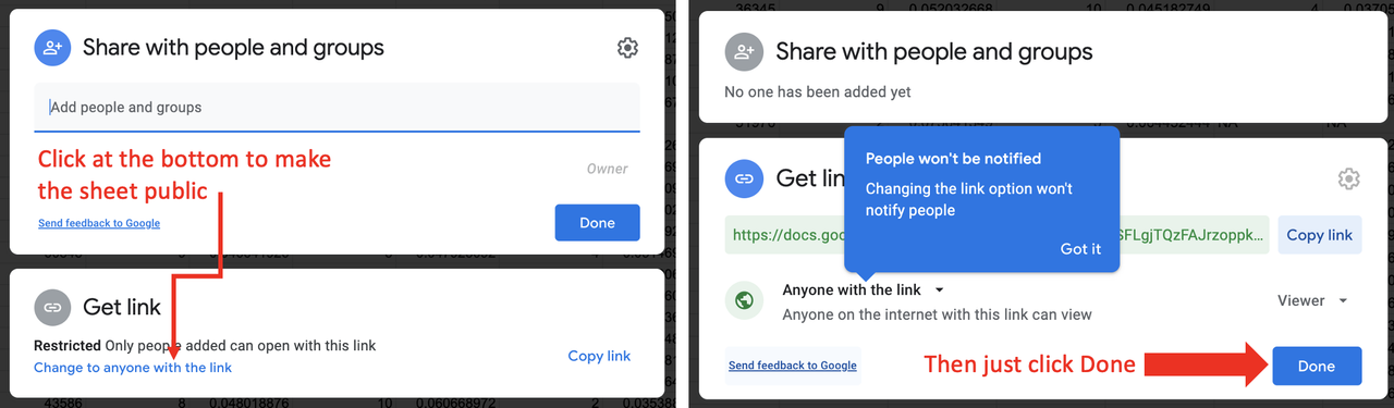
STEP 3. Make the Google Sheet public
Once you are in your own copy of the Google Sheet, click on the <Share> button in the upper right. At the bottom of the window that opens, under Get Link, click on Change to anyone with the link (see left panel of figure below). Then just click <Done> (right panel of figure).
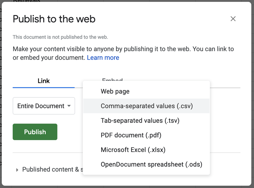
STEP 4. Go to the File menu and select Publish to the Web.
Where it says Web Page in the drop down menu, change it to Comma-separated values (.csv) (see picture). Then click the <Publish> button. This makes the data in your Google Sheet available to anyone on the internet with the link.
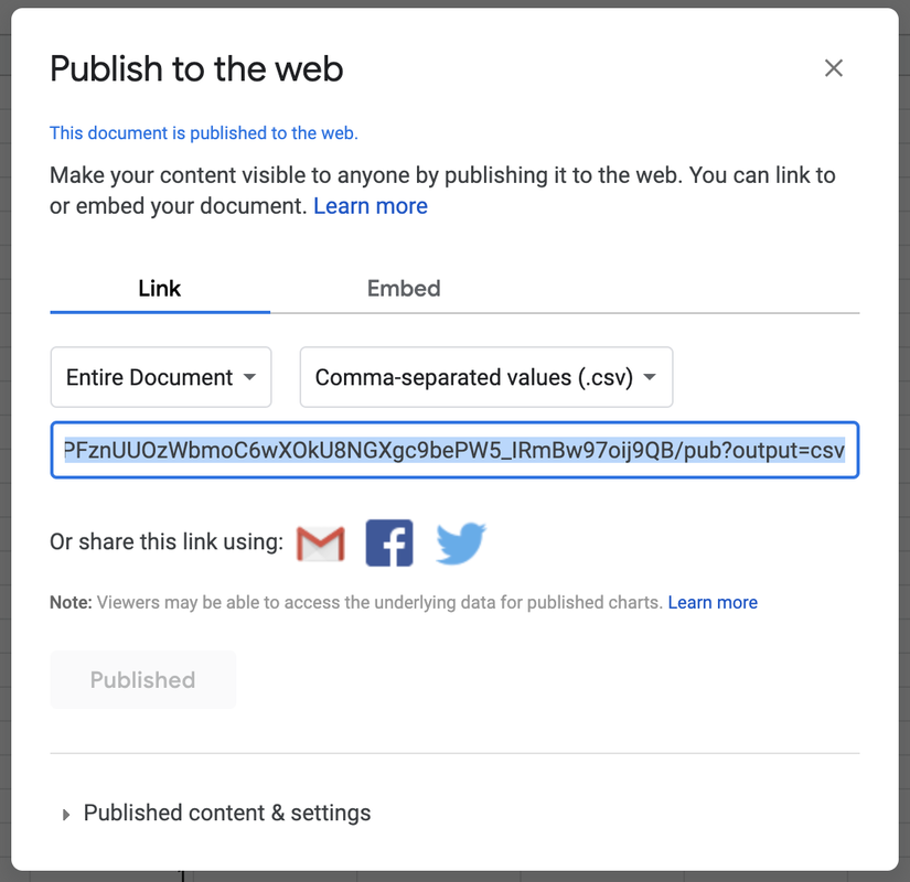
STEP 5. Copy the shareable link (highlighted in blue) to the clipboard.
STEP 6. Open your code window sandbox and run this code:
link <- "http://crazy_long_url_that_you_get_from_google"
example_data_frame <- read.csv(link, header=TRUE)
Be sure to replace the url between the quotes with your shareable link (keeping the quotes), and replace example_data_frame with a name of your choice.
Note: the header=TRUE argument indicates that the first row of the data file contains the variable names. If it doesn’t, simply omit this part of the code.
Continuing our example, let’s call the data frame deloache1997. Complete the code in the code window below to import the data into a data frame.
require(coursekata)

csvlink <- "https://docs.google.com/spreadsheets/d/e/2PACX-1vSb88NlGCW93VSbl4XiPaxf1iDPhbNDgG2FToX3MHxjr0-Bl4eAKQ9HlMoCW_Of0pXqLIfvP8AVb26L/pub?gid=1002384760&single=true&output=csv"
# This code saves the link to the google sheet into an R object named csvlink
csvlink <- "https://docs.google.com/spreadsheets/d/e/2PACX-1vSb88NlGCW93VSbl4XiPaxf1iDPhbNDgG2FToX3MHxjr0-Bl4eAKQ9HlMoCW_Of0pXqLIfvP8AVb26L/pub?gid=1002384760&single=true&output=csv"

# Save the data into a data frame called deloache1997
deloache1997 <-

# Run str() on your data frame to see what the data frame contains.
deloache1997 <- read.csv(csvlink, header = TRUE)
str(deloache1997)
ex() %>% {
    check_object(., "deloache1997") %>% check_equal()
    check_function(., "str") %>% check_arg("object") %>% check_equal()
}Once you have imported the data and created the data frame, try running str() to see what the data frame contains. You should get the output below, showing 32 observations and four variables: Age, Gender, Condition, Retrievals.
'data_frame' :  32 obs. of  4 variables:
 $ Age       : int  29 29 29 30 30 30 31 31 31 31 ...
 $ Gender    : Factor w/ 2 levels "female","male": 1 2 1 2 1 2 1 1 2 1 ...
 $ Condition : Factor w/ 2 levels "Nonsymbolic",..: 1 1 1 1 1 1 1 1 1 1 ...
 $ Retrievals: int  4 3 2 4 3 2 4 4 3 2 ...