3.10 The Data Generating Process

We can learn a lot by examining distributions of data (in histograms, boxplots, etc). But keep in mind that actual data are always from a sample (they’re the cases that actually got measured) and thus only a subset of the whole population (all cases of interest). Because data are always from a sample, we will use the phrases “sample distribution” and “distribution of data” interchangeably.

When we examine data, our interest is not only in the distribution of data, but in the population from which it was drawn. In this course, we dig a little deeper into the population. Not only do we want to use our data to help us better understand the population, but we also want to understand the processes that produced the variation in the population itself, which in turn is reflected in the data. This is what we refer to as the Data Generating Process (DGP).

If our answer to the question, “Why does the sample distribution look the way it does?” is just, “Because that’s the way the population distribution looks,” it’s not very satisfying. We would want to go on to ask, “Why does the population distribution look the way it does?” The answer to this question gets at the DGP, which is often what we are most interested in.

Whether we are examining the distribution of a single variable (like we are in this chapter), or the relationships among variables (like in the next chapter), we always want to be digging deeper, trying to understand what processes may have produced the variation we see in our data.

Example: The DGP of Bus Wait Times

Here’s a simple example. The histogram below shows the distribution of 60,000 waiting times at a bus stop on the corner of Fifth Avenue and 97th Street in New York City [source].

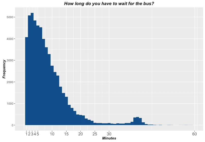
From the histogram you can see that most people wait just a short time for the bus, while some people end up waiting longer times. But to answer “why” questions requires going beyond the data in the histogram to consider the DGP.

To better understand the DGP we need to imagine the people waiting at a bus stop, and why they got there when they did. We need to activate our everyday knowledge about bus systems and how they work. Buses have schedules, and because many of the passengers are regulars who don’t want to wait at the bus stop for a long time, they roughly know when the bus will come and try to get to the bus stop just before it comes.

The Population is the Result of the DGP Over a Long Period of Time

For some data situations, it’s enough to consider the population. If you are taking a sample of likely voters in order to predict an election result, you can imagine the complete population being “out there,” just waiting to be sampled (or not). But for people waiting at a bus stop, the population is constantly shifting.

There is a deep and important relationship between the DGP and the population. The population is the long-term result of many processes, which we refer to in the aggregate as the DGP. You could think of the DGP as a lot of causal factors, each with some probability of occurrence, that produce the population distribution over time.

Because the DGP and population are related in this way, we will sometimes use the terms interchangeably. In doing so, we are emphasizing that the truth that we seek is not just about the data but about all the processes that produced the distributions we see. It includes the processes (e.g., sampling and research design) that resulted in our data, but also the processes that generated variation in the world from which the data were collected.