12.3 The Basic Idea Behind Confidence Intervals

If we extend this logic just a bit, we will be able to find the range of \(\beta_1\)s that would be likely to produce the sample \(b_1\); this is the basic idea behind confidence intervals. We’re using the word “likely” to mean that the sample \(b_1\) would be part of the middle .95 most likely samples from these DGPs.

Instead of answering a yes/no question as to whether we should reject the empty model or not, confidence intervals allow us to quantify the variation in a sample estimate and make statements such as, “We are 95% confident that the true parameter in the DGP falls between these two values.” In order to make such a statement, we need a way to find a lower bound and an upper bound for where the true value of \(\beta_1\) might be.

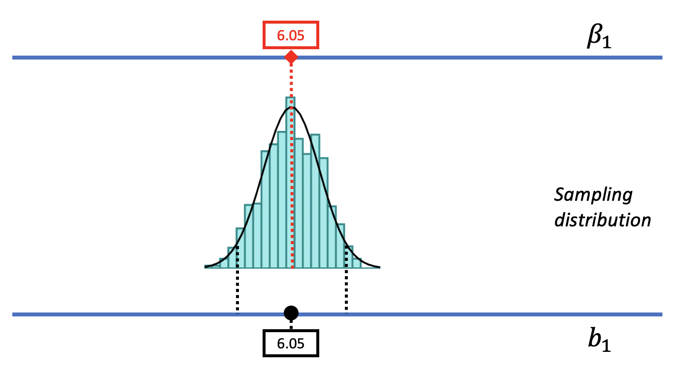
We can start by positioning the DGP and its sampling distribution centered at the sample \(b_1\) of $6.05. It makes sense to start here because \(b_1\) is the best point estimate of the DGP, and it is an unbiased estimator, meaning that the true \(\beta_1\) could be higher or could be lower, but is just as likely to be higher as it is lower.

In the picture below, we slide the DGP and its sampling distribution down (to the left), until we reach a value of the DGP where the sample \(b_1\) is about to fall into the unlikely tail. When we get down to a \(\beta_1\) of -$0.67, we can see that the sample \(b_1\) falls right at the boundary of what we would call unlikely. Thus, -$0.67 is the value of \(\beta_1\) that marks the lower bound of the 95% confidence interval.

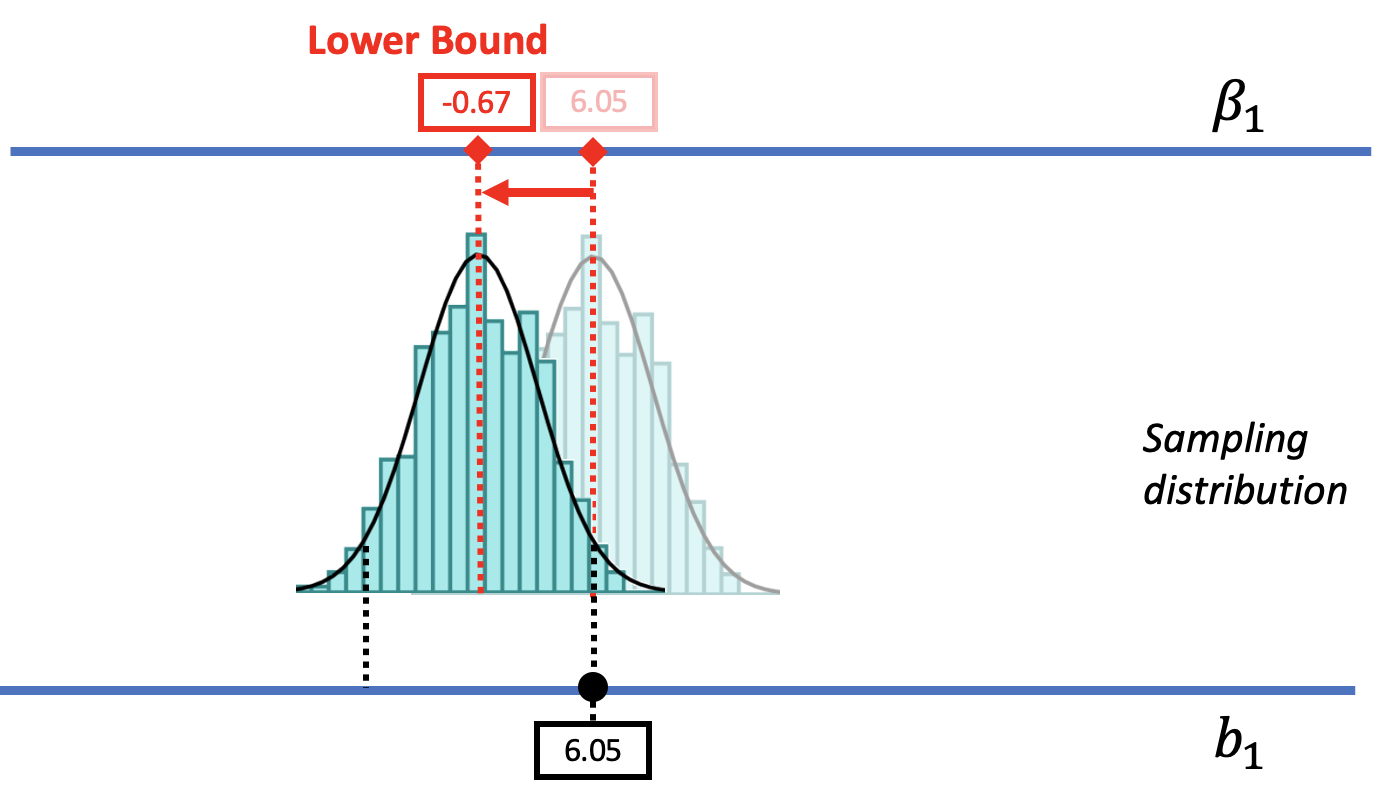
If we were to move the \(\beta_1\) lower than -0.67, the sampling distribution would also move further down and the observed \(b_1\) would become less and less likely to have been generated from these lower DGPs. In this way, we have found a lower bound for the 95% confidence interval: there is a less than .025 chance for any value of \(\beta_1\) lower than -$0.67 to have generated a sample \(b_1\) of $6.05.

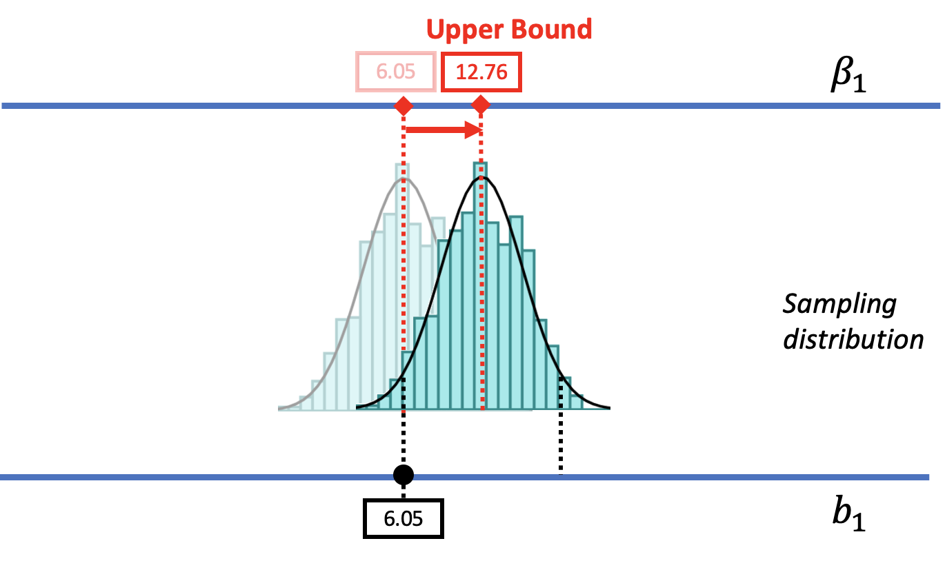
We can use a similar approach to find the upper bound of the confidence interval. As we move the DGP up (to the right), we can consider larger possible values of \(\beta_1\). At some point, as we move the sampling distribution up, we will see the sample \(b_1\) fall into the lower tail of the sampling distribution. When we get to a \(\beta_1\) of 12.76, the \(b_1\) of $6.05 falls past the cutoff into the region we would call unlikely. This value of \(\beta_1\) is considered the upper bound of the 95% confidence interval.

Putting it all together, we can illustrate the 95% confidence interval, and how it relates to the sampling distribution of \(b_1\), like this:

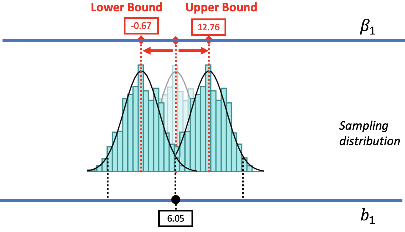
If the sample \(b_1\) has only a .025 chance of being from a DGP lower than the lower bound, and a .025 chance of being from a DGP higher than the upper bound, it follows that we can be 95% confident that the true \(\beta_1\) is somewhere between the two boundaries. This interval is the 95% confidence interval.