12.5 Using the Bootstrapped Sampling Distribution to Find the Confidence Interval
We have now succeeded in creating a bootstrapped sampling distribution of 1000 \(b_1\)s centered at the sample \(b_1\) (roughly $6.05) using the resample() function. To find the lower and upper bounds of the confidence interval, we will use our sampling distribution of \(b_1\)s as a probability distribution, interpreting proportions of \(b_1\)s falling in a certain range as a probability that future \(b_1\)s would fall into the same range.
We want to find the cutoffs that separate the middle .95 of the resampled sampling distribution from the lower and upper .025 tails because these cutoffs will correspond perfectly with the lower and upper bound of the confidence interval.
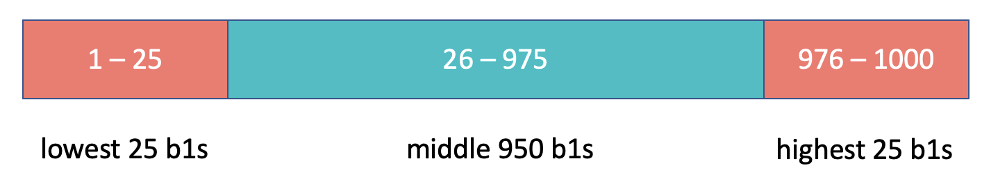
To do this, we start by putting the 1000 \(b_1\)s in order. Then we can find the cutoffs that separate the top 25 and the bottom 25 \(b_1\)s from the middle 950 \(b_1\)s.
We can visualize this task by shading in the middle .95 differently from the tails (.025 in each tail) as shown in the histogram below. (The histogram will show all the values of resampled \(b_1\) in order from smallest to largest on the x-axis.)
gf_histogram(~b1, data = sdob1_boot, fill = ~middle(b1, .95), bins = 80)
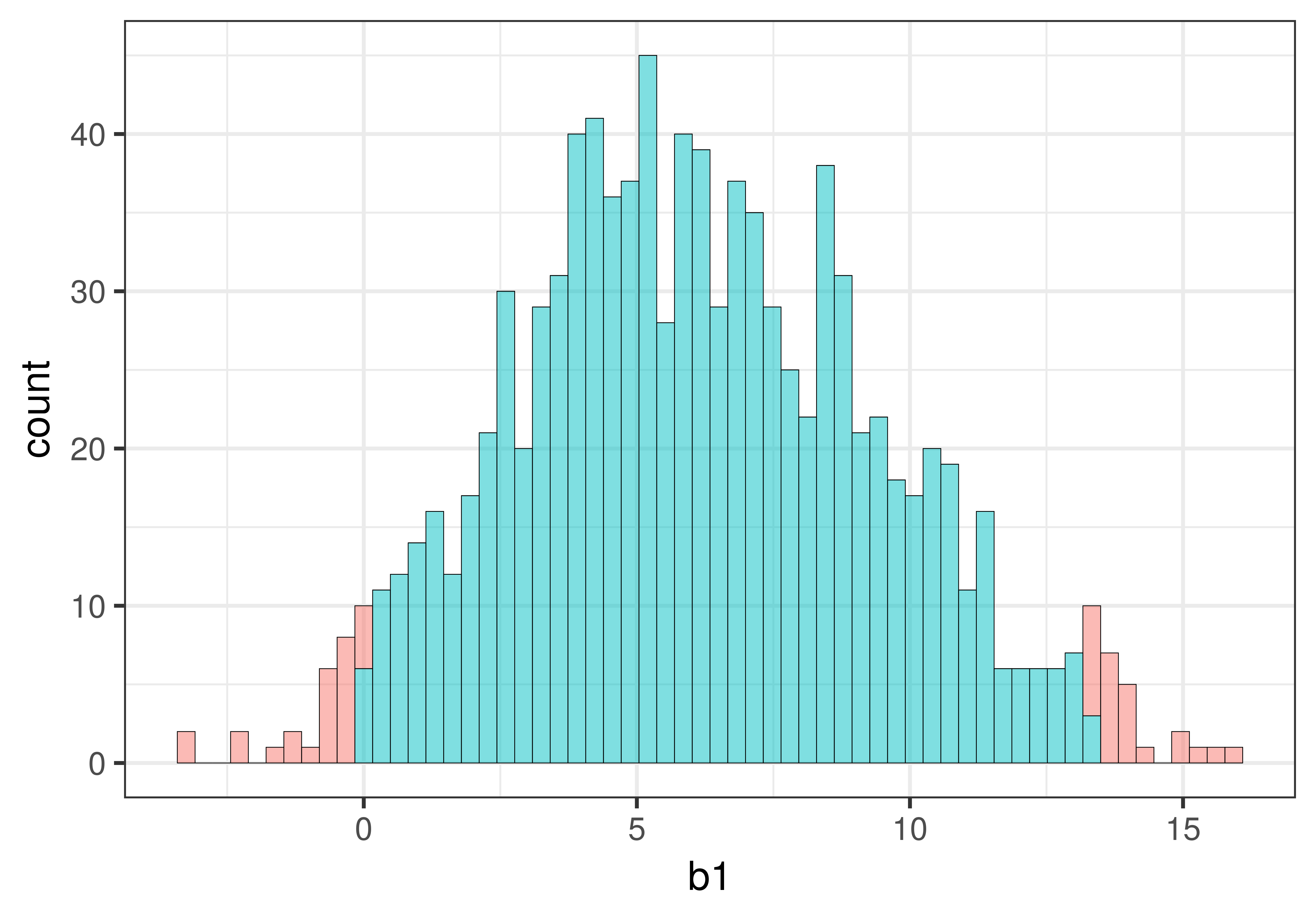
As illustrated below, the cutoff for the lowest .025 of \(b_1\)s is at the 26th \(b_1\). The cutoff for the highest .025 of \(b_1\)s is at the 975th \(b_1\). These two cutoffs correspond to the lower and upper bound of the confidence interval.
Here’s some code that will arrange the \(b_1\)s in order (from lowest to highest) and save the re-arranged data back into sdob1_boot.
sdob1_boot <- arrange(sdob1_boot, b1)To identify the 26th b1 in the arranged data frame (26th from the lowest), we can use these brackets (e.g., [26]).
sdob1_boot$b1[26]Use the code block below to print out both the 26th and 975th b1s.
require(coursekata)

sdob1_boot <- do(1000) * b1(Tip ~ Condition, data = resample(TipExperiment))
sdob1_boot <- arrange(sdob1_boot, b1)
# we’ve written code to print the 26th b1
sdob1_boot$b1[26]

# write code to print the 975th b1
# we’ve written code to print the 26th b1
sdob1_boot$b1[26]

# write code to print the 975th b1
sdob1_boot$b1[975]
ex() %>% {
      check_output_expr(., "sdob1_boot$b1[26]")
      check_output_expr(., "sdob1_boot$b1[975]")
}
[1] -0.02484472
[1] 13.3Based on our bootstrapped sampling distribution of \(b_1\), the 95% confidence interval runs from around 0 to 13 (give or take). Your numbers will be slightly different from ours, of course, because they are generated randomly. Based on this analysis, we can be 95% confident that the true value of \(\beta_1\) in the DGP lies in this range.