Course Outline
-
segmentGetting Started (Don't Skip This Part)
-
segmentStatistics and Data Science: A Modeling Approach
-
segmentPART I: EXPLORING VARIATION
-
segmentChapter 1 - Welcome to Statistics: A Modeling Approach
-
segmentChapter 2 - Understanding Data
-
segmentChapter 3 - Examining Distributions
-
3.12 From DGP to Population to Samples
-
segmentChapter 4 - Explaining Variation
-
segmentPART II: MODELING VARIATION
-
segmentChapter 5 - A Simple Model
-
segmentChapter 6 - Quantifying Error
-
segmentChapter 7 - Adding an Explanatory Variable to the Model
-
segmentChapter 8 - Digging Deeper into Group Models
-
segmentChapter 9 - Models with a Quantitative Explanatory Variable
-
segmentPART III: EVALUATING MODELS
-
segmentChapter 10 - The Logic of Inference
-
segmentChapter 11 - Model Comparison with F
-
segmentChapter 12 - Parameter Estimation and Confidence Intervals
-
segmentChapter 13 - What You Have Learned
-
segmentFinishing Up (Don't Skip This Part!)
-
segmentResources
list High School / Advanced Statistics and Data Science I (ABC)
3.12 From DGP to Population to Samples
A Long-Run of Our DGP
Now that we have made an R program to simulate the DGP of rolling a dice one time, we can try using it to roll a dice 10, 100, 1,000, or even 10,000 times. On first glance, you might think we could just revise the code for rolling a dice once to have it roll the dice 10 times: sample(dice_outcomes, 10) But this won’t work.
The reason it doesn’t work is that we are asking R to randomly sample 10 numbers when there are only 6 numbers in the vector! The sample() function, by default, samples without replacement. When it has sampled one number, that number is no longer available (i.e., not replaced back in the vector) to be sampled again. We can tell R to sample with replacement by adding in the additional argument replace = TRUE like this: sample(dice_outcomes, 10, replace = TRUE).
Try running the broken code in the code block below. Then add the code to tell R to sample with replacement.
require(coursekata);
dice_outcomes <- c(1, 2, 3, 4, 5, 6)

# fix this line of code
my_sample <- sample(dice_outcomes, 10)

# this prints out my_sample
my_sample
dice_outcomes <- c(1, 2, 3, 4, 5, 6)

# fix this line of code
my_sample <- sample(dice_outcomes, 10, replace = TRUE)

# this prints out my_sample
my_sample
ex() %>% {
    override_solution_code(.,
        'dice_outcomes <- c(1, 2, 3, 4, 5, 6); my_sample <- sample(dice_outcomes, 10, replace = TRUE); # this prints out my_sample
my_sample'
    )
    } %>% {
    check_object(., "my_sample") %>% check_equal()
}
(There is another R function that samples with replacement, called resample(). It’s the same as adding replace=TRUE as an argument to the sample() function. You can try it out if you want in the code window above. As usual, there are many ways to accomplish the same thing in R.)
We have simulated 10 rolls of the dice, but that hardly would count as the “long run” required to approximate a population. In the code block below, edit the code to generate 1,000 dice rolls and save it in a new vector called large_sample. Then create a bar graph of the distribution of dice rolls in large_sample. What shape do you expect to see in the bar graph?
require(coursekata)
dice_outcomes <- c(1, 2, 3, 4, 5, 6)

# edit this to generate a sample of 1000 dice rolls
large_sample <- sample( )

# create a bar graph of large_sample
dice_outcomes <- c(1, 2, 3, 4, 5, 6)

# edit this to generate a sample of 1000 dice rolls
large_sample <- sample(dice_outcomes, 1000, replace = TRUE)

# create a bar graph of large_sample
gf_bar(~ large_sample)
ex() %>% override_solution_code('{
dice_outcomes <- c(1, 2, 3, 4, 5, 6)

# edit this to generate a sample of 1000 dice rolls
large_sample <- sample(dice_outcomes, 1000, replace = TRUE)

# create a bar graph of large_sample
gf_bar(~ large_sample)
}') %>% {
    check_object(., "large_sample") %>% check_equal()
    check_function(., "gf_bar") %>%
        check_arg("object") %>%
        check_equal(eval = FALSE)
}
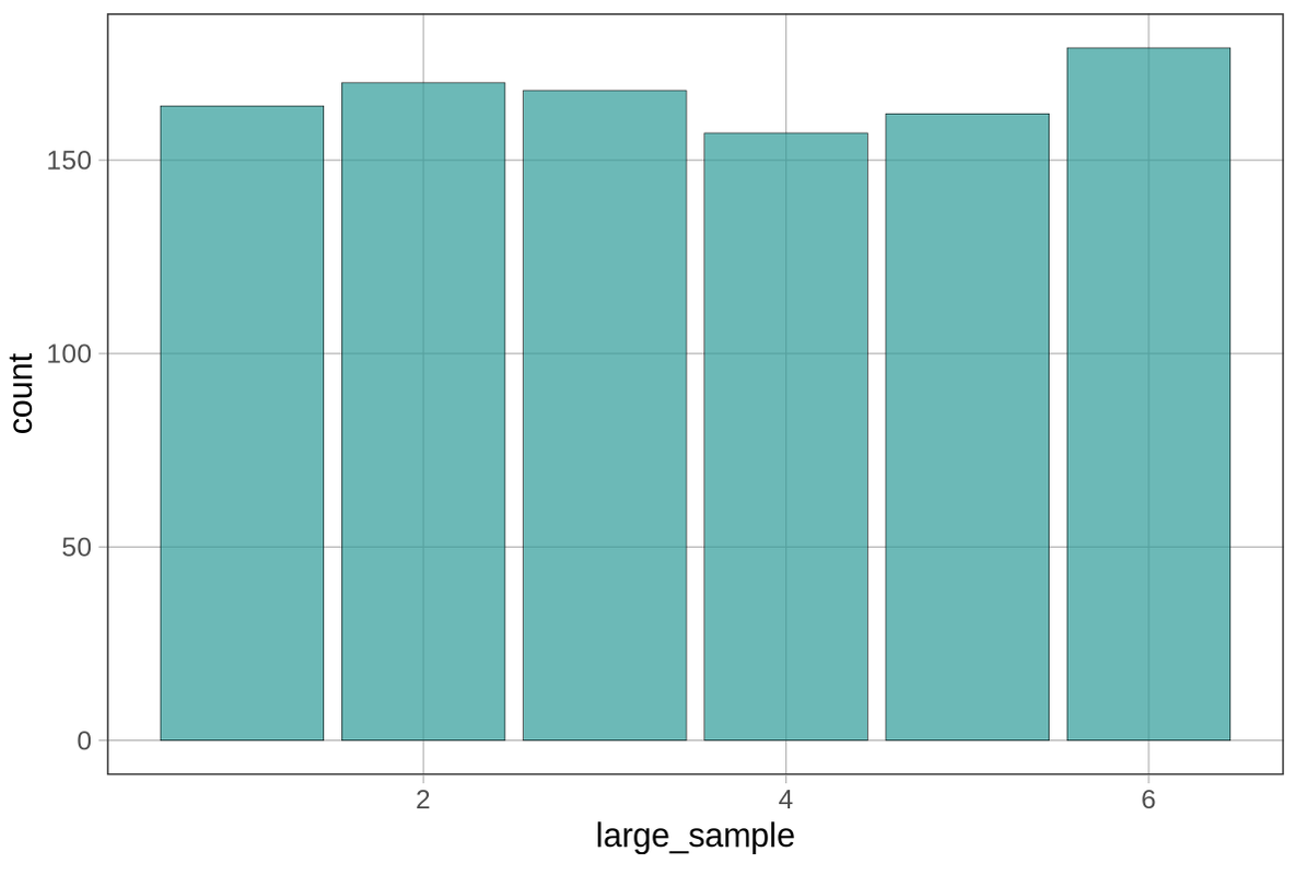
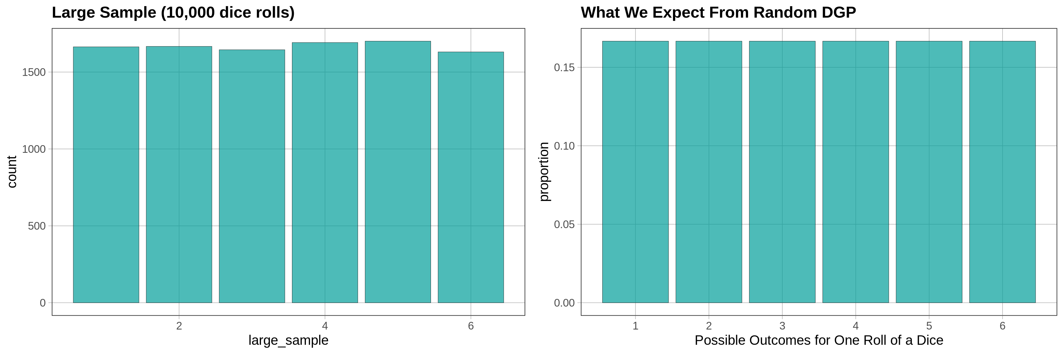
This larger sample looks a lot more like what we would expect the distribution of dice rolls to look like. Try simulating an even larger sample by running your DGP 10,000 times. The more times we run the DGP, the more it starts to look like what we expected to see.
When you run a DGP (e.g., sampling with replacement, or resampling, from the numbers 1 to 6) for a long time (e.g., 10,000 times), you end up with a distribution that we can start to call a population. But even if you only roll the dice one time, the DGP is still the same. This is why we distinguish between the population and the DGP.
Large Samples Versus Small Samples
Large samples are pretty good at representing a population distribution and the DGP. For example, we saw that larger samples, of 1,000 or 10,000 die rolls, showed a uniform distribution with each outcome being roughly equally probable, just as we would predict based on our understanding of the DGP for rolling a die.
But what about small samples? For practical reasons, we often have only a small sample of data, perhaps only 100 or 24 or 12 observations. How well do small samples reflect the population distribution?
Examining Variation Across Smaller Samples
Let’s use our random DGP of dice rolls to produce smaller samples. We can sample with replacement by adding the argument replace = TRUE or by simply using the resample() function.
Try using resample() to create a sample of 100 dice rolls. Add some code to create a bar graph of the results.
require(coursekata)
dice_outcomes <- 1:6

# edit this to create a sample of 100 dice rolls
my_sample <- resample()

# Write code to create a bar graph of my_sample
dice_outcomes <- 1:6

# edit this to create a sample of 100 dice rolls
my_sample <- resample(dice_outcomes, 100)

# Write code to create a bar graph of my_sample
gf_bar(~ my_sample)
ex() %>% {
override_solution_code(.,
'dice_outcomes <- 1:6; my_sample <- resample(dice_outcomes, 100); gf_bar(~ my_sample)'
) %>% {
check_object(., "my_sample") %>% check_equal()
check_function(., "gf_bar") %>% {
check_arg(., "object") %>% check_equal(eval = FALSE)
}
}
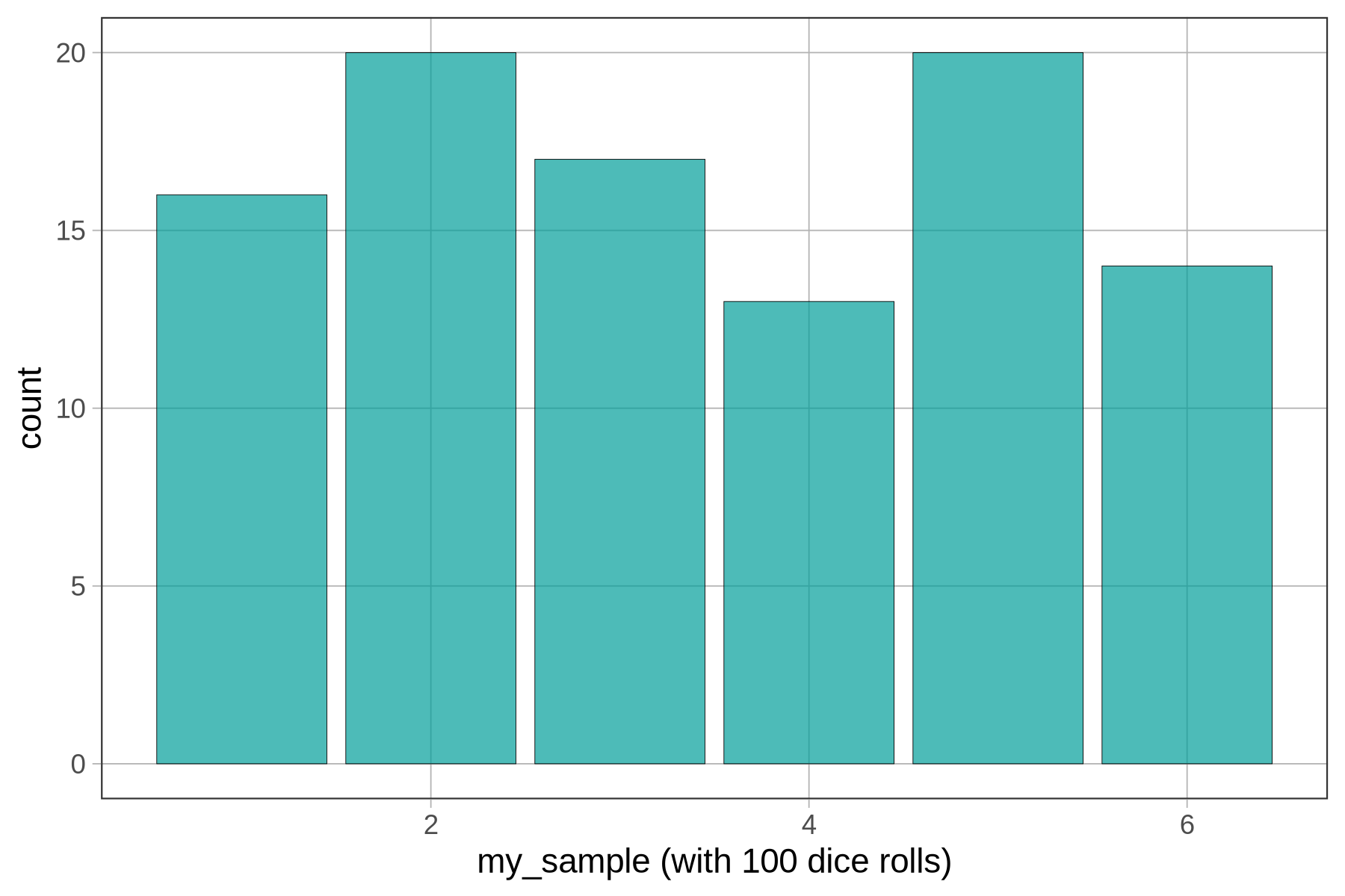
}Here is one of the random samples we generated. Your random sample will look different from ours, of course, because it’s random! Notice that neither your sample nor ours looks very much like the uniform distribution we would expect based on our knowledge of the DGP.
Now let’s take an even smaller sample of just 12 die rolls. Modify the code below to simulate 12 die rolls and save it as a vector called my_sample. What do you think the distribution of this sample will look like? How closely will it resemble the uniform distribution we might expect?
require(coursekata)
dice_outcomes <- 1:6

# simulate 12 dice rolls with resample and save it as my_sample


# this will create a bar graph of my_sample
gf_bar(~ my_sample)
dice_outcomes <- 1:6

# simulate 12 dice rolls with resample and save it as my_sample
my_sample <- resample(dice_outcomes, 12)

# this will create a bar graph of my_sample
gf_bar(~ my_sample)
ex() %>% {
    override_solution_code(.,
        'dice_outcomes <- 1:6; my_sample <- resample(dice_outcomes, 12); gf_bar(~ my_sample)'
    ) %>% {
        check_object(., "my_sample") %>% check_equal()
        check_function(., "gf_bar") %>% {
            check_arg(., "object") %>% check_equal(eval = FALSE)
        }
    }
}
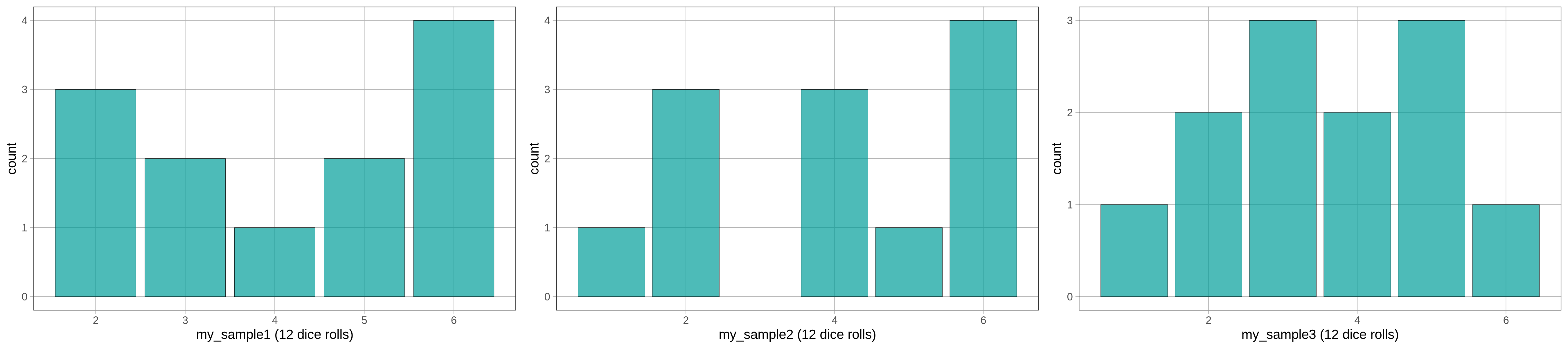
We’ve depicted three different samples of 12 die rolls. Notice that our randomly generated sample distributions are not perfectly uniform. In fact, they may not look very uniform to our eyes at all! You might even be asking yourself, is this really a random process? Even if you simulate 12 die rolls a few more times (try pressing <Run> a few times), most of the distributions won’t look very uniform.
The fact is, each of these samples were generated by a random data generating process: simulated die rolls. And even though we know this process would produce a uniform population distribution over the long run, our samples of 12 or 100 dice don’t usually look uniform.
The important point to understand is that sample distributions can vary, even a lot, from the underlying population distribution from which they are drawn. This is what we call sampling variation. Small samples (even samples of 100 are considered “small”) will not necessarily look like the population they are drawn from, even if they are drawn purely by random.