12.2 Thinking With Sampling Distributions

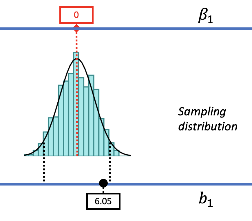
Up to now, we have centered all of our thinking with sampling distributions around the empty model. In Chapters 9 and 10, we always started by assuming that \(\beta_1\) is 0 and then went on to make sampling distributions based on this assumption. In this chapter we will move beyond the empty model and consider other models that could have produced the sample \(b_1\).

Our basic strategy is illustrated in the animated gif below. We start with the same sampling distribution we constructed based on the empty model. But then, using our hypothetical thinking skills, we mentally move the sampling distribution up and down along the number line, imagining different possible values of \(\beta_1\).

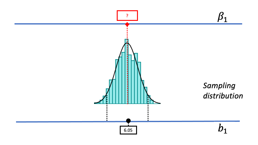
As we begin thinking about alternative models of the DGP, we will assume that the shape and spread of the sampling distribution stays constant across different hypothesized values of \(\beta_1\). By making these assumptions, it makes it possible for us to use a sampling distribution created based on one particular DGP (e.g., the empty model) for other DGPs up and down the scale. Later we will provide more justification for this assumption, but for now just go with us!

As we mentally move the sampling distribution up and down the measurement scale we consider different possible values of \(\beta_1\). For each of these possible values we ask the same question we asked using the sampling distribution centered at a \(\beta_1\) of 0: Given the new hypothesized value of \(\beta_1\), is such a DGP likely to generate our sample \(b_1\)?

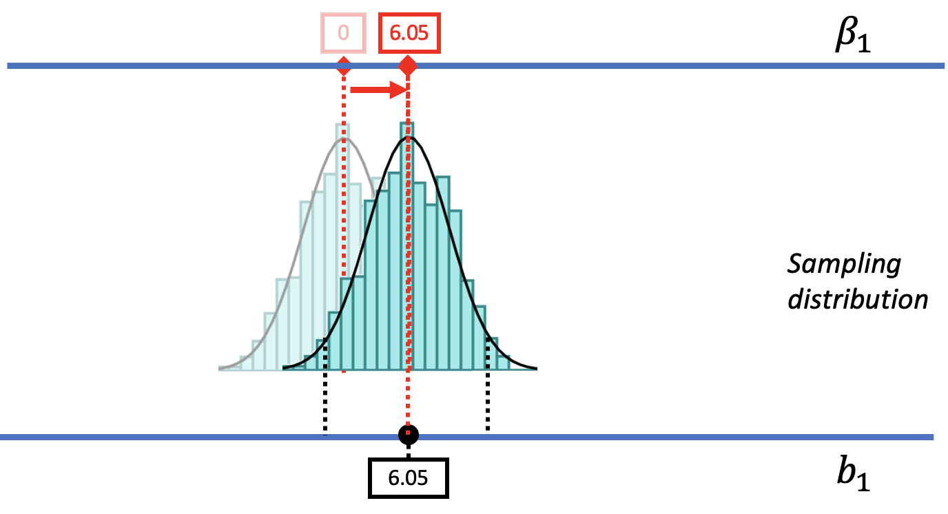
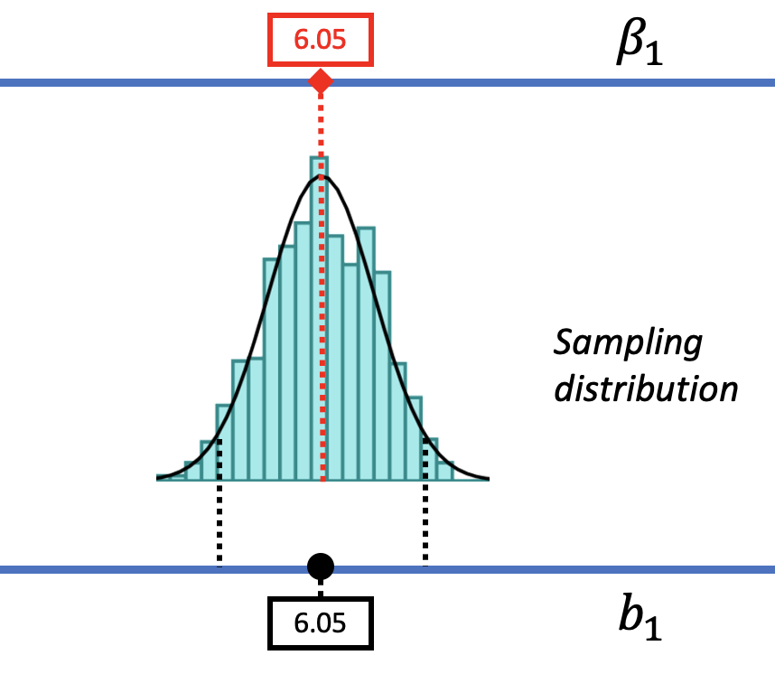
Let us show you what we mean. In the figure below we have moved the sampling distribution we constructed based on the empty model for the tipping study up (to the right) until it is centered at a DGP where \(\beta_1=6.05\). We now pose the question, “If the true \(\beta_1\) is $6.05, is our sample \(b_1\) of $6.05 likely?

We saw before that a DGP in which \(\beta_1=0\) could produce the observed sample \(b_1\) of $6.05. That was our reason for not rejecting the empty model. But that does not mean the true \(\beta_1\) in the DGP is actually 0. The pictures above show it’s also possible that the true \(\beta_1\) is $6.05! And $6.05 was, after all, the best-fitting estimate of \(\beta_1\) based on the data.

From our musings so far, we can see that \(\beta_1\) could be 0 or it could be $6.05. But these are just two of the many possible DGPs that could have produced the sample estimate of $6.05. Once we start imagining different possible DGPs, and the sampling distributions each would generate, we will see more and more possibilities.

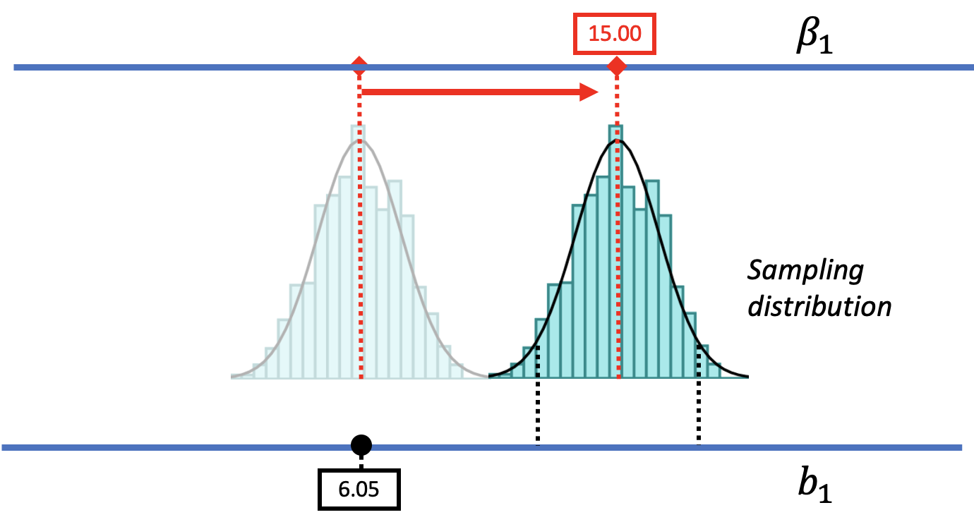
But using this strategy, we can also rule out some possibilities. There are values of \(\beta_1\) that are not likely to produce the sample estimate. Imagine a DGP with a \(\beta_1\) a lot larger than $6.05; for example, a world where the true difference between groups is 15.00. To represent this world, we could slide the DGP as well as its corresponding sampling distribution further to the right (see the picture below).

Such a DGP could produce a variety of samples. But notice that the sample \(b_1\) of $6.05 is no longer in the middle .95 region – now it’s in the lower unlikely tail. We could say, therefore, that a DGP with \(\beta_1=15.00\) is unlikely to have generated the sample \(b_1\) because $6.05 is much lower than most of the \(b_1\)s generated by this DGP.

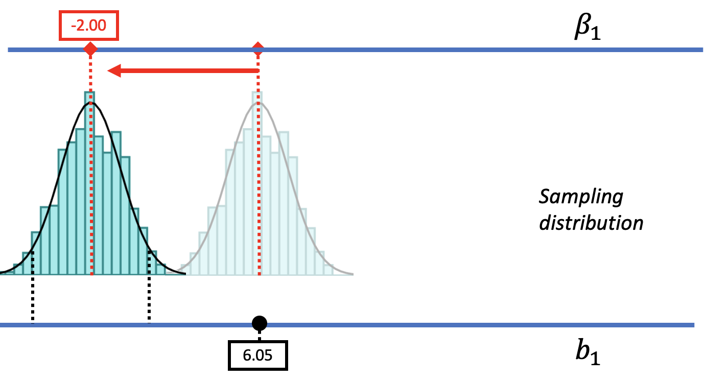
By the same logic, if we slide the sampling distribution far down to the left (as in the figure below), we can see that it is unlikely that the \(b_1\) of $6.05 came from a DGP with a \(\beta_1\) as low as -2.00. By sliding the sampling distribution left and right, we can begin to see the range of possible \(\beta_1\)s that could have generated our sample \(b_1\).