11.5 Calculating P-Value from the Sampling Distribution of F

To calculate the exact p-value, we can use the tally() function, using the proportion of our 1000 simulated Fs as extreme or more extreme than the observed F, to estimate of the probability of generating such an F if the empty model is true.

f > sample_F
 TRUE FALSE
0.081 0.919

The resulting p-value (about .08) is larger than the alpha criterion of .05, meaning that the sample F is not in the the region we have defined as unlikely. (Note that your estimate of p-value may be a little different from ours because each is based on a different set of 1000 randomly generated Fs.)

Based on this p-value, we would probably not reject the empty model of Tip. It’s possible that even if the empty model is true (that is, \(\beta_1 = 0\) and \(\text{PRE} = 0\)), we still might have observed an F just by random chance as high as the one actually observed (3.30)

P-Value Calculated from Sampling Distribution of \(b_1\) versus F

In the prior chapter we pointed out that the p-value for the effect of Condition in the tipping experiment could also be found in the ANOVA table produced by the supernova() function. Here it is again.

supernova(lm(Tip ~ Condition, data = TipExperiment))

Analysis of Variance Table (Type III SS)
Model: Tip ~ Condition

                              SS df      MS     F    PRE     p
----- ----------------- -------- -- ------- ----- ------ -----
Model (error reduced) |  402.023  1 402.023 3.305 0.0729 .0762
Error (from model)    | 5108.955 42 121.642
----- ----------------- -------- -- ------- ----- ------ -----
Total (empty model)   | 5510.977 43 128.162

Notice that the p-value of .0762 is close to the p-value we just calculated using the sampling distribution of F, and also is close to the p-value we obtained in the previous chapter using the sampling distribution of \(b_1\). This is not an accident. The reason these p-values are similar is because they are testing the same thing – the effect of smiley face on Tip – using different methods.

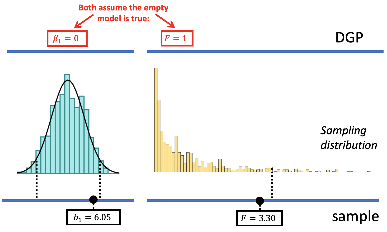
We have now used shuffle() to construct sampling distributions for three sample statistics: \(b_1\), PRE, and F. By using shuffle(), we were simulating a DGP in which the empty model is true, i.e., that whether or not a smiley face is drawn on the check does not affect how much a table tips. The variation we see in the sampling distributions is assumed to be due to random sampling variation.

The shapes of the sampling distributions are different for \(b_1\) than for F (see figure below). The sampling distribution of \(b_1\) is roughly normal in shape, while the one for F has a distinctly asymmetric shape, with a long tail off to the right. The rejection region defined by alpha is split between two tails for the sampling distribution of \(b_1\), but is all in the upper tail of the sampling distribution of F.

Once we constructed the sampling distribution, we used it to put the observed sample statistic in context. Specifically, it enabled us to ask how likely it would be to select a sample with a sample statistic – be it \(b_1\), PRE, or F – as extreme or more extreme as the statistic observed in the sample. The answer to this question is the p-value.

We can use the p-value to decide, based on our stated alpha of .05, whether the observed sample statistic would be unlikely or not if the empty model is true. If we judge it to be unlikely (i.e., p < .05), then we would most likely decide to reject the empty model in favor of the more complex model. But if the p-value is greater than .05, which it is for the Condition model of Tip, we would probably decide to stick with the empty model for now, pending further evidence.