Course Outline
-
segmentGetting Started (Don't Skip This Part)
-
segmentStatistics and Data Science: A Modeling Approach
-
segmentPART I: EXPLORING VARIATION
-
segmentChapter 1 - Welcome to Statistics: A Modeling Approach
-
segmentChapter 2 - Understanding Data
-
segmentChapter 3 - Examining Distributions
-
segmentChapter 4 - Explaining Variation
-
segmentPART II: MODELING VARIATION
-
segmentChapter 5 - A Simple Model
-
segmentChapter 6 - Quantifying Error
-
segmentChapter 7 - Adding an Explanatory Variable to the Model
-
segmentChapter 8 - Digging Deeper into Group Models
-
segmentChapter 9 - Models with a Quantitative Explanatory Variable
-
segmentPART III: EVALUATING MODELS
-
segmentChapter 10 - The Logic of Inference
-
segmentChapter 11 - Model Comparison with F
-
segmentChapter 12 - Parameter Estimation and Confidence Intervals
-
12.7 Using the t-Distribution to Construct a Confidence Interval
-
segmentChapter 13 - What You Have Learned
-
segmentFinishing Up (Don't Skip This Part!)
-
segmentResources
list High School / Advanced Statistics and Data Science I (ABC)
12.7 Using the t-Distribution to Construct a Confidence Interval
Just as we used the t-distribution in the previous chapter to model the sampling distribution of \(b_1\) for purposes of calculating a p-value (the approach used by supernova()), we can use it here to calculate a 95% confidence interval.
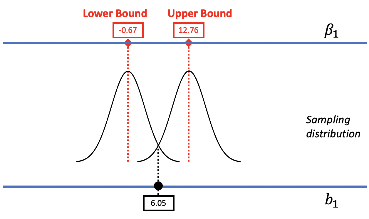
In the figure below, we replaced the resampled sampling distribution of \(b_1\)s with one modeled by the smooth t-distribution with its associated standard error. As before, we can mentally move the t-distribution down and up the scale to find the lower and upper bounds of the confidence interval.
The R function that calculates a confidence interval based on the t-distribution is confint().
Here’s the code you can use to directly calculate a 95% confidence interval that uses the t-distribution as a model of the sampling distribution of \(b_1\):
confint(lm(Tip ~ Condition, data = TipExperiment))The confint() function takes as its argument a model, which results from running the lm() function. In this case we simply wrapped the confint() function around the lm() code. You could accomplish the same goal using two lines of code, the first to create the model, and the second to run confint(). Try it in the code block below.
require(coursekata)
# create the condition model of tip and save it as Condition_model
Condition_model <-
confint(Condition_model)
# create the condition model of tip and save it as Condition_model
Condition_model <- lm(Tip ~ Condition, data = TipExperiment)
confint(Condition_model)
ex() %>%
  check_function("lm") %>%
  check_result() %>%
  check_equal()
2.5 % 97.5 %
(Intercept) 22.254644 31.74536
ConditionSmiley Face -0.665492 12.75640
As you can see, the confint() function returns the 95% confidence interval for the two parameters we are estimating in the Condition model. The first one, labelled Intercept, is the confidence interval for \(\beta_0\), which we remind you is the mean for the Control group. The second line shows us what we want here, which is the confidence interval for \(\beta_1\).
Using this method, the 95% confidence interval for \(\beta_1\) is from -0.67 to 12.76. Let’s compare this confidence interval to the one we calculated above on the previous page using bootstrapping: 0 to 13. While these two confidence intervals aren’t exactly the same, they are darn close, which gives us a lot of confidence. Even when we use very different methods for constructing the confidence interval, we get very similar results.
Margin of Error
One way to report a confidence interval is to simply say that it goes, for example, from -0.67 to 12.76. But another common way of saying the same thing is to report the best estimate (6.05) plus or minus the margin of error (6.72), which you could write like this: \(6.05 \pm 6.72\).
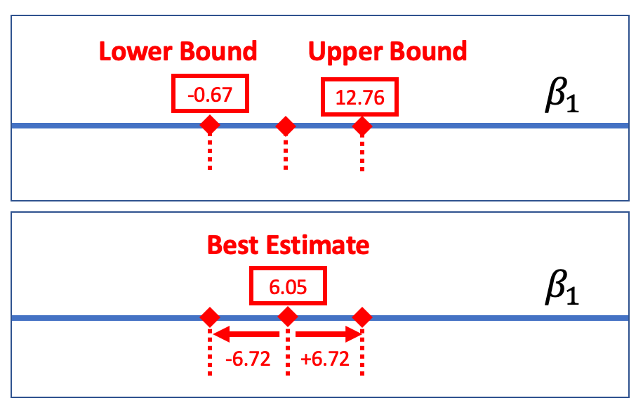
The margin of error is the distance between the upper bound and the sample estimate. In the case of the tipping experiment this would be \(12.76 - 6.05\), or $6.72. If we assume that the sampling distribution is symmetrical, the margin of error will be the same below the parameter estimate as it is above.
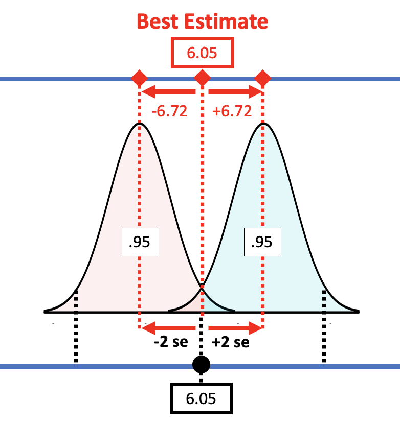
We can always calculate the margin of error by using confint() to get the upper bound of the confidence interval and then subtracting the sample estimate. But we can do a rough calculation of margin of error using the empirical rule. According to the empirical rule, 95% of all observations under a normal curve fall within plus or minus 2 standard deviations from the mean.
Applying this rule to the sampling distribution, the picture below shows that the margin of error is approximately equal to two standard errors. If we start with a t-distribution centered at the sample \(b_1\), we would need to slide it up about two standard errors to reach the cutoff above which \(b_1\) (6.05) falls into the lower .025 tail.
If you have an estimate of standard error, you can simply double it to get the approximate margin of error. If, for example, we use the standard error generated by R (3.33) for the condition model, the margin of error would be twice that, or 6.66. That’s pretty close to the margin of error we calculated from confint(): 6.72.
R uses the Central Limit Theorem to estimate standard error, but we also have other ways of getting the standard error. Using shuffle() to create the sampling distribution resulted in a slightly larger standard error of 3.5. If we double that, we get a margin of error of 7, slightly larger than the 6.66 we got using R’s estimate of standard error. In general, if the standard error is larger, the margin of error will be larger and so will the confidence interval.