12.12 Confidence Intervals for Pairwise Comparisons

In a previous chapter we discussed testing the pairwise comparisons in a three-group model. We looked at some data comparing students’ outcomes on a math test after playing three different educational games. We first used an F test to compare the three-group model with the empty model, and decided to reject the empty model (that the outcomes from all three games could be modeled with the same average score).

Knowing that at least some of the three games differed statistically from each other, but not knowing which ones, we conducted pairwise comparisons, testing the three possible pairings of the three games, A, B, and C.

Here is the code we used to conduct the pairwise comparisons for the game_model:

pairwise(game_model)

And here is the output, on which we added some yellow highlighting:

Model: outcome ~ game

game

Levels: 3

Family-wise error-rate: 0.05

  group_1 group_2  diff pooled_se     q    df  lower upper p_adj
                   
1 B       A       2.086     0.516 4.041   102  0.350 3.822 .0142
2 C       A       3.629     0.516 7.031   102  1.893 5.364 .0000
3 C       B       1.543     0.516 2.990   102 -0.193 3.279 .0920

Note that the p-values and the confidence intervals are adjusted (hence reported as p_adj) based on Tukey’s Honestly Significant Difference test to maintain an overall (or family-wise) Type I error rate of 0.05.

The mean difference between B and C in the sample is 1.54. But the p-value of .09 tells us that the observed difference is within the range of differences we would consider likely if the true difference between the games were 0. For this reason, we did not reject the empty model for this pairwise difference.

Because we have learned that model comparison (using the p-value) and confidence intervals are related, we would expect this finding to be mirrored in the 95% confidence interval. Specifically, because we did not reject the empty model based on the p-value, we should expect that the confidence interval would include 0, meaning that a \(\beta_1\) of 0 is one of a range of models we would consider likely to have generated the sample \(b_1\).

As shown below, the confidence interval of the difference between games C and B is centered at the sample difference (1.54) but extends from -0.19 to 3.28. As expected based on the p-value (greater than .05), this interval includes 0.

  group_1 group_2  diff pooled_se     q    df  lower upper p_adj
                   
1 B       A       2.086     0.516 4.041   102  0.350 3.822 .0142
2 C       A       3.629     0.516 7.031   102  1.893 5.364 .0000
3 C       B       1.543     0.516 2.990   102 -0.193 3.279 .0920

Try Adding plot=TRUE to the pairwise() Function

The pairwise() function has an option to help us visualize the pairwise confidence intervals in relation to each other. Just add the argument plot = TRUE to the function, like this:

pairwise(game_model, plot = TRUE)

Try it in the code window below.

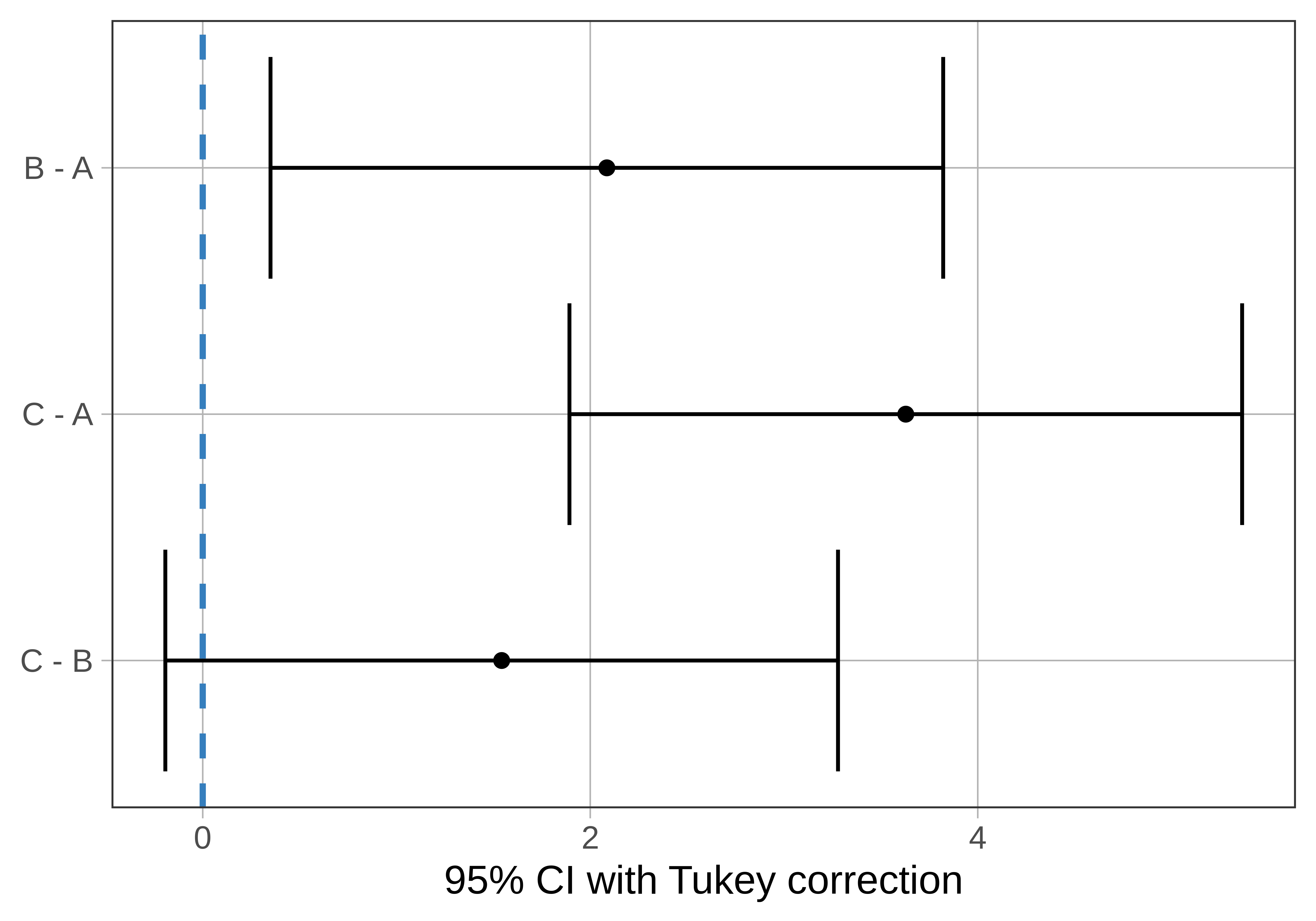
Notice that one of the 95% confidence intervals crosses the dotted line, which represents a pairwise difference of 0: C and B. But the other two confidence intervals (C - A and B - A) do not include 0. This means that we are not confident that the mean difference in the DGP for these pairs could be 0. We would conclude that game A is indeed different from both games B and C in the DGP.