12.4 Using Bootstrapping to Calculate the 95% Confidence Interval

Sliding a visualization up and down is a good way to understand the concept behind confidence intervals, but it’s not a very good way to calculate the actual upper and lower bounds! In this section we will learn one method (among many) to calculate a confidence interval.

In sliding the sampling distribution around, we’re making a few assumptions. We assume, first, that the shape and spread of the sampling distribution does not change as we slide it up and down the measurement scale. The sampling distribution is roughly normal for \(b_1\), which means it is unimodal and symmetrical, with a tail on either end.

We are also going to assume that the center of the confidence interval is at the observed sample \(b_1\) (e.g., $6.05 in the tipping study). We can convince you of this, we hope, using the picture below. We have re-colored the sampling distribution centered at $6.05 in red. We also drew in two dotted black lines indicating the cutoffs that separate the likely and unlikely area of that sampling distribution. Behind it are the distributions we used to find the upper and lower bounds.

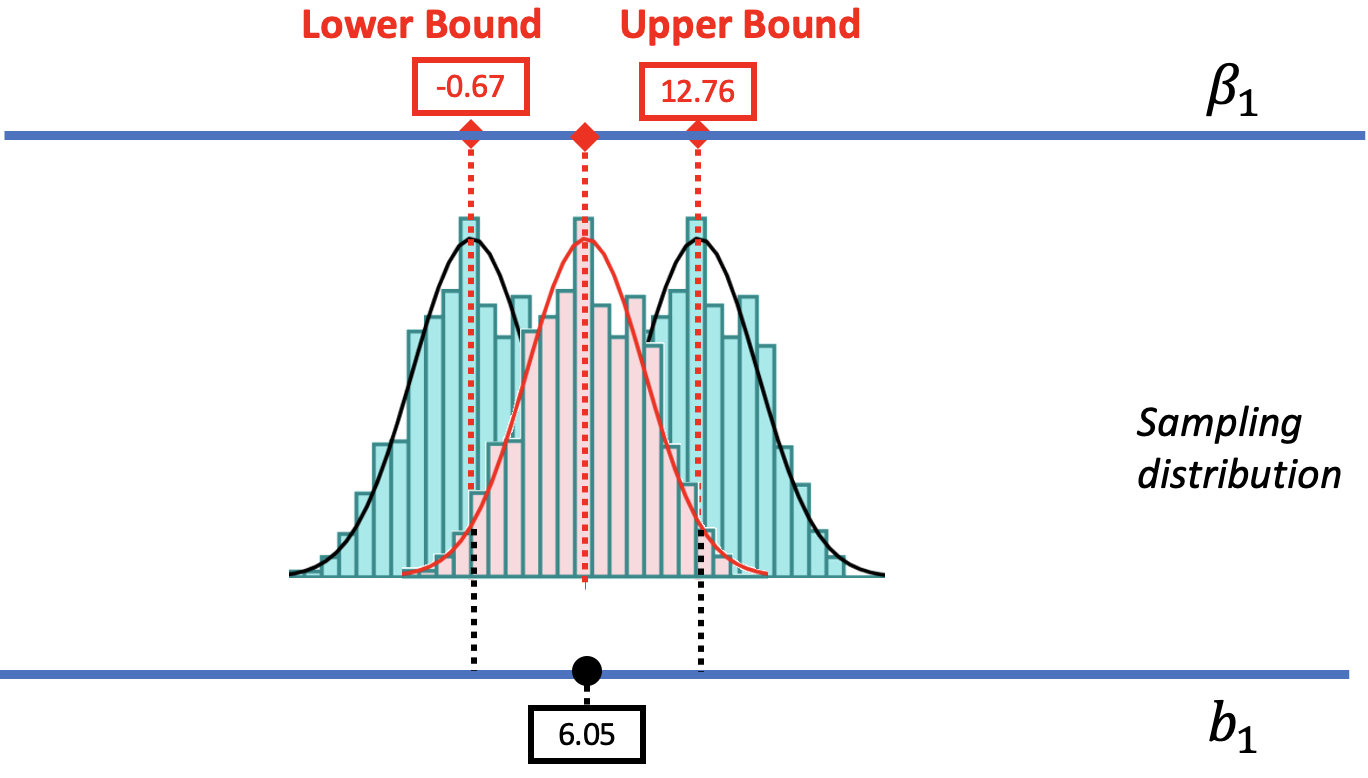
The .025 cutoff in the lower tail of the sampling distribution centered at the sample \(b_1\) lines up perfectly with the lower bound of the confidence interval. Likewise, the .025 cutoff in the upper tail lines up with the upper bound of the confidence interval. If only we had a sampling distribution centered at \(b_1\), we would be able to figure out the lower and upper bounds.

Bootstrapping with resample()

For calculating the confidence interval, it would be helpful to have a sampling distribution centered at the sample \(b_1\). Unfortunately, the shuffle() function, which mimics a DGP where \(\beta_1=0\), produces a sampling distribution that is centered at 0. But we need to mimic a DGP where the \(\beta_1\) is equal to our sample \(b_1\) (6.05).

We can do this using the resample() function. The resample() function assumes that the entire population of interest is made up of observations that look just like the ones in our sample. In the case of the tipping experiment, we would assume a population made up of many copies of the tables in the TipExperiment sample.

By repeatedly sampling from this imaginary population, we can create a sampling distribution of \(b_1\)s that will be centered at the observed sample \(b_1\). This approach to creating a sampling distribution is sometimes called bootstrapping.

We previously used the resample() function with a vector (just a list of numbers) to simulate dice rolls. In bootstrapping, we will resample cases from a data frame instead of numbers from a vector.

To illustrate how this works, let’s focus on a subgroup of 6 tables from the TipExperiment data frame. We have put these six tables in a new data frame called SixTables. The output below shows the contents of this data frame.

  TableID Tip   Condition
        4  34     Control
       18  21     Control
       43  21 Smiley Face
        6  31     Control
       25  47 Smiley Face
       35  27 Smiley Face

Notice that in our small sample of 6 tables, there are 3 tables in the Smiley Face condition and 3 in the Control condition.

Now let’s see what happens when we resample() from this sample of 6 tables.

resample(SixTables)

In the table below, we’ve put the original 6 tables on the left, and the results of the resample() function on the right.

  TableID Tip   Condition
        4  34     Control
       18  21     Control
       43  21 Smiley Face
        6  31     Control
       25  47 Smiley Face
       35  27 Smiley Face

  TableID Tip   Condition
       43  21 Smiley Face
        6  31     Control
       18  21     Control
        6  31     Control
       18  21     Control
       35  27 Smiley Face

The resample() function takes a new random sample of six tables from the data set. It samples with replacement, meaning that when R randomly samples a table, it then puts the table back so it could potentially be sampled again. This explains why a table in the original data might appear more than once, or perhaps not at all, in the resampled data.

Okay, enough already with just six tables!

Let’s now use resample() to bootstrap a new sample of 44 tables from the tables in the tipping study. Later, we will repeat this process many times to bootstrap a sampling distribution of \(b_1\)s. Let’s start by thinking about what would happen if you ran the following line of code on the complete TipExperiment data frame:

resample(TipExperiment)

Both the resampled and original data frames will have 44 tables. However, because some tables might be selected more than once in the resampled data frame, and others not at all, the number of tables in each condition won’t exactly match the numbers in the original data frame. (We aren’t going to worry about this for now.)

We can also see that the average Tip for each condition will be different in the resampled data frame. This makes sense because the exact tables included are not the same in the two data frames.

Use the code window below to produce the \(b_1\) estimate for the Condition model of Tip in both the original and resampled data frames. Run the code a few times, and see what you notice.

Each time you run the code you will get two \(b_1\)s printed out. The first is based on the original data frame, and will always be $6.05; we know this by now! But the second \(b_1\) will vary each time you run the code. This is because each time you run the code, R is calculating the mean difference between smiley face and control group in a new resampled version of the data frame.