Course Outline
-
segmentGetting Started (Don't Skip This Part)
-
segmentStatistics and Data Science: A Modeling Approach
-
segmentPART I: EXPLORING VARIATION
-
segmentChapter 1 - Welcome to Statistics: A Modeling Approach
-
segmentChapter 2 - Understanding Data
-
segmentChapter 3 - Examining Distributions
-
3.5 The Five-Number Summary
-
segmentChapter 4 - Explaining Variation
-
segmentPART II: MODELING VARIATION
-
segmentChapter 5 - A Simple Model
-
segmentChapter 6 - Quantifying Error
-
segmentChapter 7 - Adding an Explanatory Variable to the Model
-
segmentChapter 8 - Digging Deeper into Group Models
-
segmentChapter 9 - Models with a Quantitative Explanatory Variable
-
segmentPART III: EVALUATING MODELS
-
segmentChapter 10 - The Logic of Inference
-
segmentChapter 11 - Model Comparison with F
-
segmentChapter 12 - Parameter Estimation and Confidence Intervals
-
segmentChapter 13 - What You Have Learned
-
segmentFinishing Up (Don't Skip This Part!)
-
segmentResources
list High School / Advanced Statistics and Data Science I (ABC)
3.5 The Five-Number Summary
So far we have used histograms as our main tool for examining distributions. But histograms aren’t the only tool we have available. In this section we will introduce a few more tools for examining distributions of quantitative variables. Later in this chapter, we will also introduce some tools for examining the distributions of categorical variables.
Sorting Revisited, and the Min/Max/Median
In the previous chapter we introduced the simple idea of sorting a quantitative variable in order. Before sorting the numbers, it was hard to see a pattern. You could read the numbers, but it was hard to draw any conclusions about the distribution itself.
As soon as we sort the numbers in order, we can see things that are true of the distribution. For example, when we sort even a long list of numbers we can see what the smallest number is and what the largest number is. This shows us something about the distribution that we couldn’t have seen just by looking at a jumbled list of numbers.
We can demonstrate this by looking at the Wt variable in the MindsetMatters data frame. Write some code to sort the housekeepers by weight from lowest to highest, and then see what the minimum and maximum weights are.
require(coursekata)
# Write code to sort Wt from lowest to highest
# Write code to sort Wt from lowest to highest
arrange(MindsetMatters, Wt)

# Alternative solution
sort(MindsetMatters$Wt)
3
ex() %>% check_or(
    check_function(., "arrange", not_called_msg = "If you were trying to use `sort`, that's acceptable but your code must have resulted in an error.") %>% check_result() %>% check_equal(),
    check_function(., "sort") %>% check_result() %>% check_equal()
)
[1] 90 105 107 109 115 115 115 117 117 118 120 123 123 124 125 126 127
[18] 128 130 130 131 133 134 134 135 136 137 137 137 140 140 141 142 142
[35] 142 143 144 145 145 148 150 150 154 154 155 155 156 156 156 157 158
[52] 159 160 161 161 161 162 163 163 164 166 167 167 168 170 172 173 173
[69] 178 182 183 184 187 189 196Note that you can also use the function arrange() to sort, but that will sort the entire data frame. We just wanted to be able to see the sorted weights in a row, so we just used sort() on the vector (MindsetMatters$Wt).
Now that we have sorted the weights, we can see that the minimum weight is 90 pounds and the maximum weight is 196 pounds. In addition to knowing the minimum and maximum weight, it would be helpful to know what the number is that is right in the middle of this distribution. If there are 75 housekeepers, we are looking for the 38th housekeeper’s weight, because there are 37 weights that are smaller than this number and 37 that are bigger than this number. This middle number is called the median.
Numbers such as the minimum (often abbreviated as min), median, and maximum (abbreviated as max) are helpful for understanding a distribution. These three numbers can be thought of as a three-number summary of the distribution. We’ll build up to the five-number summary in a bit.
There is a function called favstats() (for favorite statistics) that will quickly summarize these values for us. Here is how to get the favstats for Wt from MindsetMatters.
favstats(~ Wt, data = MindsetMatters) min Q1 median Q3 max mean sd n missing
90 130 145 161.5 196 146.1333 22.46459 75 0There are a lot of other numbers that are generated by the favstats() function, but let’s take a look at Min, Median, and Max for now. By looking at the median weight in relation to the minimum and maximum weight, you can tell a little bit about the shape of the distribution.
Try writing code to get the favstats() for the variable Population for countries in the data frame HappyPlanetIndex.
require(coursekata)

HappyPlanetIndex$Region <- recode(
    HappyPlanetIndex$Region,
    '1'="Latin America",
    '2'="Western Nations",
    '3'="Middle East and North Africa",
    '4'="Sub-Saharan Africa",
    '5'="South Asia",
    '6'="East Asia",
    '7'="Former Communist Countries"
)
# Modify the code to get favstats for Population of countries in HappyPlanetIndex
favstats()
# Modify the code to get favstats for Population of countries in HappyPlanetIndex
favstats(~ Population, data = HappyPlanetIndex)
ex() %>% check_function("favstats") %>% check_result() %>% check_equal() min Q1 median Q3 max mean sd n missing
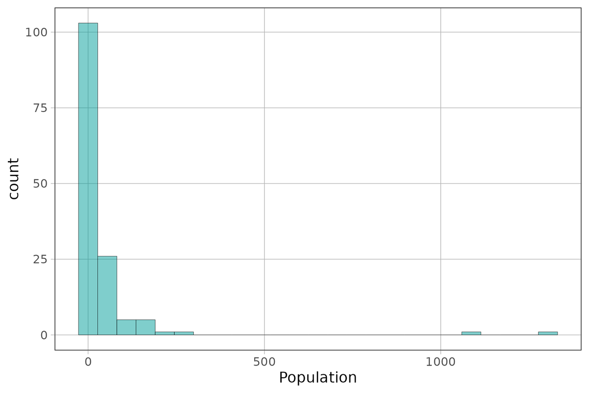
0.29 4.455 10.48 31.225 1304.5 44.14545 145.4893 143 0Create a histogram of Population to see if your intuition about the shape of this distribution from looking at the min/median/max is correct.
require(coursekata)

HappyPlanetIndex$Region <- recode(
    HappyPlanetIndex$Region,
    '1'="Latin America",
    '2'="Western Nations",
    '3'="Middle East and North Africa",
    '4'="Sub-Saharan Africa",
    '5'="South Asia",
    '6'="East Asia",
    '7'="Former Communist Countries"
)
# make a histogram of Population from HappyPlanetIndex using gf_histogram
# make a histogram of Population from HappyPlanetIndex using gf_histogram
gf_histogram(~ Population, data = HappyPlanetIndex)
ex() %>% check_or(
    check_function(., "gf_histogram") %>% {
    check_arg(., "object") %>% check_equal()
    check_arg(., "data") %>% check_equal()
},
    override_solution(., "gf_histogram(HappyPlanetIndex, ~ Population)") %>%
    check_function("gf_histogram") %>% {
    check_arg(., "object") %>% check_equal()
    check_arg(., "gformula") %>% check_equal()
},
    override_solution(., "gf_histogram(~HappyPlanetIndex$Population)") %>%
    check_function("gf_histogram") %>% {
    check_arg(., "object") %>% check_equal()
},
    override_solution(., "gf_histogram(data = HappyPlanetIndex, gformula = ~ Population)") %>%
    check_function("gf_histogram") %>% {
    check_arg(., "data") %>% check_equal()
    check_arg(., "gformula") %>% check_equal()
}
    )