11.2 Sampling Distribution of PRE

Just as finding a difference between the two means (e.g., $6.05) does not by itself rule out the possibility that the true difference in the DGP could be 0, the same is true of PRE. The two-group model of Tip reduces error by .07 in the data. But that doesn’t rule out the possibility that the true PRE in the DGP might be 0.

If there is no difference between the groups in the DGP, then none of the error from the empty model would be reduced by the two group model that includes Condition. That is if \(\beta_1=0\), then the true value of PRE in the DGP would also be 0. One follows from the other.

Even if the true PRE in the DGP is 0, the PRE calculated by fitting a model to a sample of data would not necessarily be 0. It would vary due to random sampling variation. As before, the question of how much it might vary is one we can answer by constructing a sampling distribution of PRE based on the empty model.

If the sample PRE falls in the unlikely region, we would probably decide to reject the empty model and to adopt the complex model. But if the sample PRE falls in the not unlikely .95 region of the sampling distribution, we might decide to not reject the empty model, as the data we collected would be judged consistent with a DGP in which PRE is 0.

It is important to note that the question we are asking using the sampling distribution of PRE is the same one we asked using the sampling distribution of \(b_1\): in both cases we want to know how likely it is that the sample statistic we observed could have been generated just by chance assuming that the empty model is true.

Saying “the true PRE = 0” is just one more way to refer to the empty model of the DGP. It’s the same as saying that there is no effect of smiley face, or that \(\beta_1=0\). Using the sampling distribution of PRE should, therefore, lead to similar results as using the sampling distribution of \(b_1\). Let’s construct a sampling distribution and find out if it does!

Constructing a Sampling Distribution of PRE

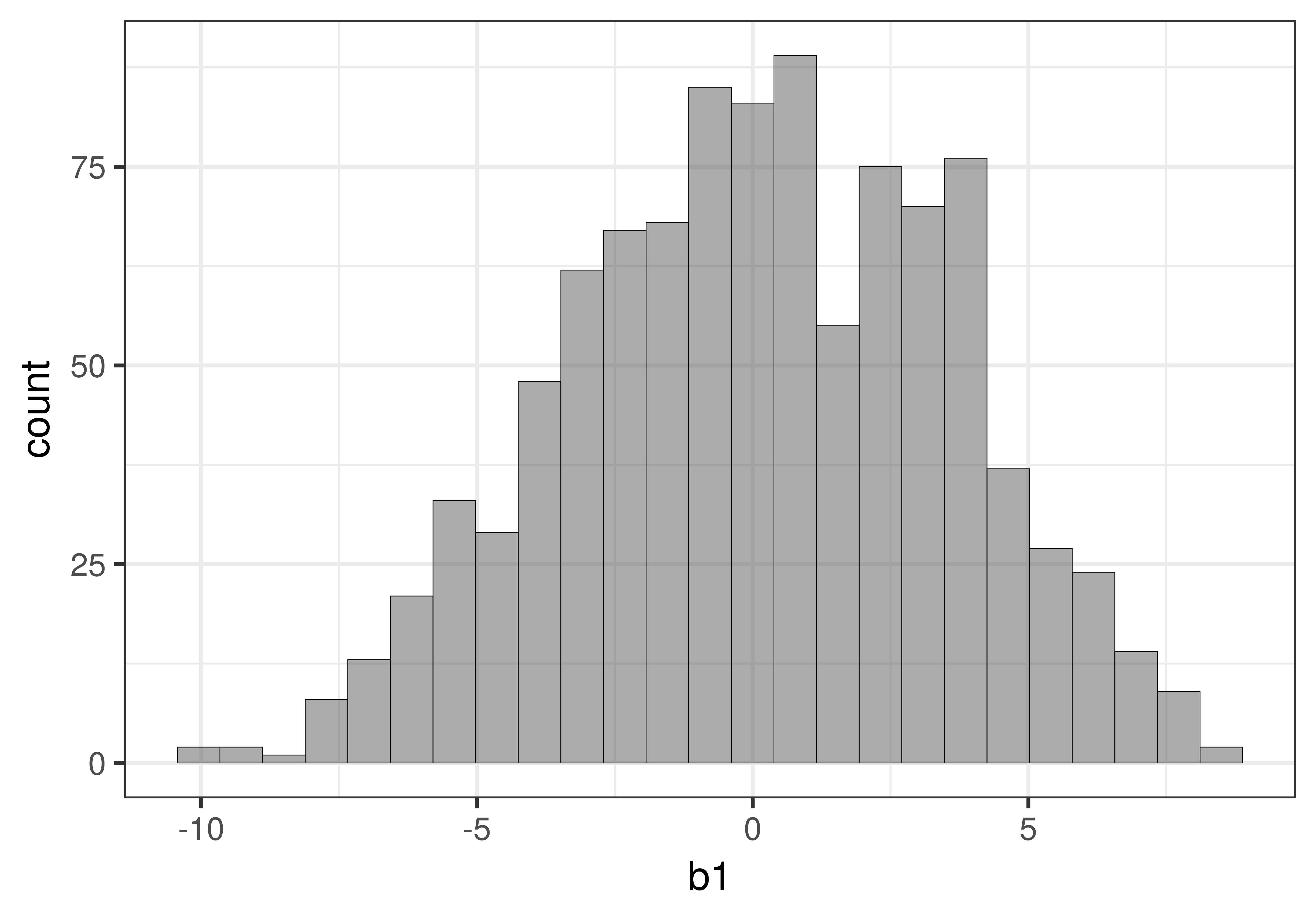
Let’s bring back a picture from the prior chapter to remind us how we used shuffle() to generate a sampling distribution of \(b_1\) assuming \(\beta_1=0\). By showing us the distribution of possible \(b_1\)s that the empty model of the DGP could have produced, the sampling distribution provided a context within which we could interpret the observed mean difference between the smiley face and no smiley face conditions ($6.05).

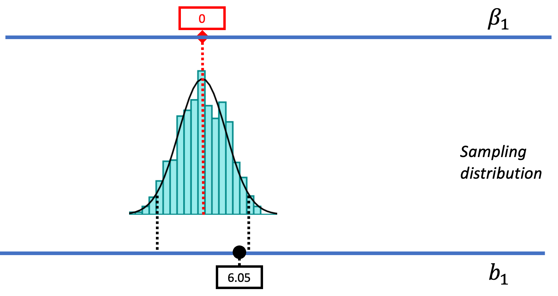
We can use the same approach to creating the sampling distribution of PRE. We will start by using shuffle() to randomize the relationship between Condition and Tip, then, instead of calculating \(b_1\), we will calculate PRE for the shuffled sample. By using shuffle() we are simulating a world where the empty model is true and where each table would have tipped the same amount regardless of which condition it was assigned to.

The line of R code below will (1) shuffle the values of Tip, (2) create a model of the shuffled Tip using Condition as the explanatory variable, and then (3) calculate the PRE of the model. It does all this for a single shuffled (or randomized) set of data.

pre(shuffle(Tip) ~ Condition, data = TipExperiment)

Modify the code in the window below to generate 10 shuffled PREs.

            pre
1  0.1122759121
2  0.0014887642
3  0.0062726047
4  0.0284102391
5  0.0056457566
6  0.0006969561
7  0.0545399059
8  0.0404193284
9  0.0356684799
10 0.0034682844

We can see that the purely random DGP in which there is no effect of smiley face on Tip produces a variety of PREs.

Let’s extend the code above to create a sampling distribution of 1000 PREs, save them into a new data frame that we will call sdoPRE (for sampling distribution of PRE), and then print out the first six rows of the data frame.

          pre
1 0.002577500
2 0.013398877
3 0.043751521
4 0.021976798
5 0.003006396
6 0.014355646

Examining the Sampling Distribution of PRE

The process we used to create the sampling distribution of PREs is similar to the one we used in the prior chapter to create a sampling distribution of \(b_1\)s. In both cases we used the shuffle() function to simulate the empty model of the DGP.

Does the sampling distribution of PRE look similar to the sampling distribution of \(b_1\)? Let’s find out! Use the code window below to make a histogram of the randomly generated PREs in the sdoPRE data frame.

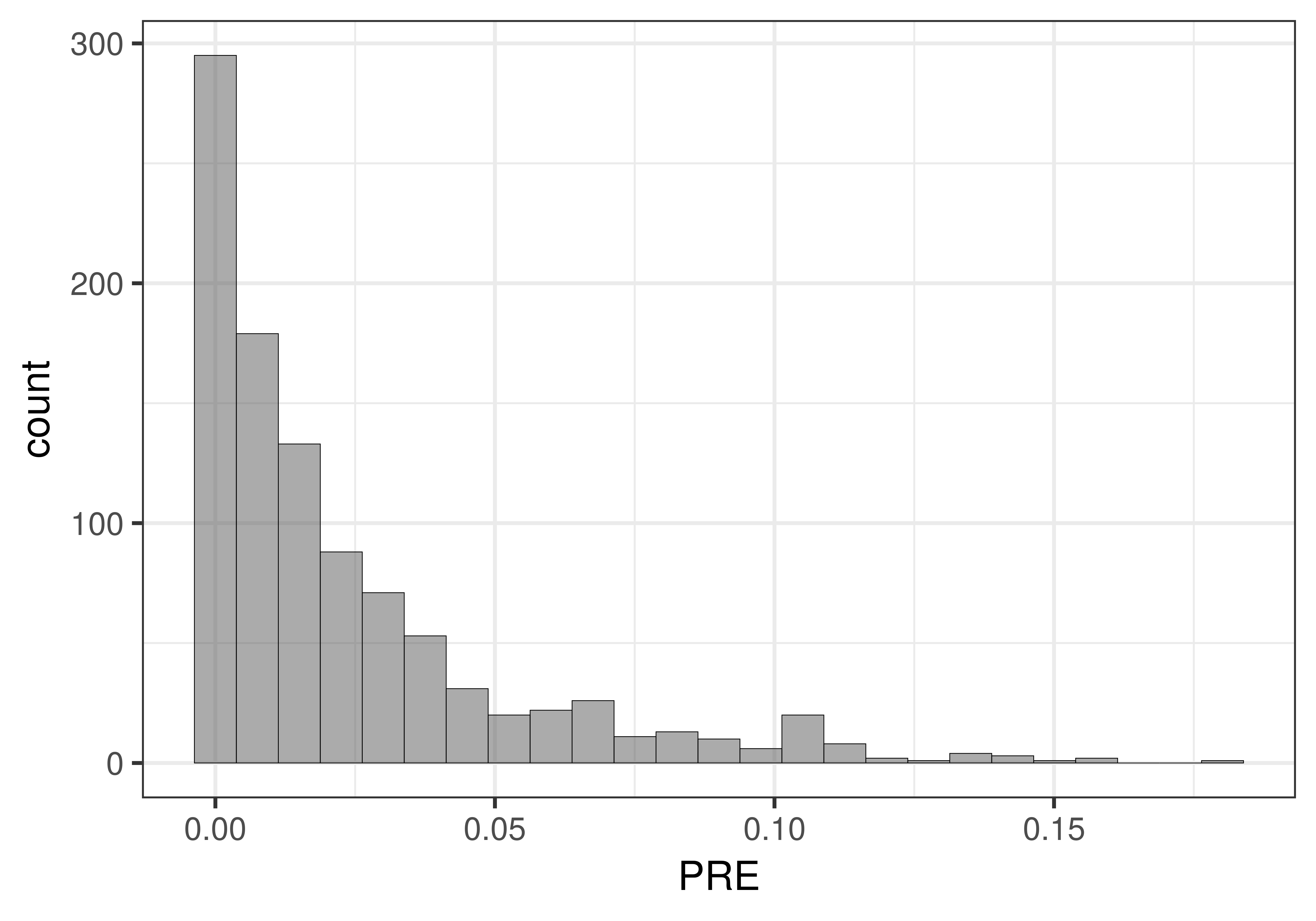
Interestingly, the sampling distribution of PRE has a very different shape than the sampling distribution of \(b_1\). In the figure below we put the two sampling distributions side by side for purposes of comparison.

The sampling distribution of \(b_1\) has two tails because the difference between the two conditions could be positive or could be negative: Smiley face could have resulted in more tips, or could have resulted in fewer tips. Both are possible (though the researchers no doubt expected it would result in more tips).

But PRE is different: The complex model can explain none of the error from the empty model (0), or all of the error from the empty model (1.0). But it cannot explain less than 0 error. Because PRE is a proportion, it has a clear lower bound of 0, and a clear upper bound of 1.

Assuming the empty model is true, the only place an extreme PRE could fall is in the upper tail of the distribution, which is why there is only one tail. An extreme positive effect of smiley face or an extreme negative effect of smiley face are both the same to PRE: both would fall in the upper tail of the sampling distribution of PRE.