11.13 The Chi-Square Test of Independence

Up to now we have used only quantitative variables as our outcome. Group models were used when the explanatory variable was categorical, regression models when the explanatory variable was quantitative. But in both cases, the outcome was quantitative.

There are other models that have been developed to apply in cases with a categorical outcome variable. We won’t cover most of these models in this book, but we will pause to look at one such model: the chi-square model, usually known as the chi-square test of independence.

Do Students Like Playing One Game More Than Another?

Let’s return to the game_data data frame. Recall that this data set reported the learning outcomes of 105 fifth-graders who were randomly assigned to play one of three games: A, B, or C. In our previous analysis we found that the students learned more from game C than from either of the other two games.

But how much did they enjoy playing the games? If students learned more from game C, but didn’t like playing it, it might not be the best type of game over the long term, because they might lose interest in playing it.

It turns out there is another variable in the data set that directly addresses this possibility. After playing the game, each student was asked: “Would you like to play again?” They could answer either yes or no, and their answers are saved in the variable play_again. We might consider the hypothesis that the variation in how students answered play_again could be explained by which game they played. Here’s the word equation for that hypothesis:

play again = game + error

Here’s a table that shows the number of students who answered yes or no after playing the game, broken down by which game they played. We ran this code to get the table:

tally(play_again ~ game, data=game_data)

         game
play_again  A  B  C
       no  16 11 19
       yes 19 24 16

On examining the table, it looks like our fears might, in fact, be confirmed: Although students learn more from game C, that’s the only one of the three games after which the majority of students (19 out of 35) say, “No,” they would rather not play again.

Expected Frequencies Under the Empty Model

Of course, the differences across games in whether students want to play again could just be an artifact of sampling variation. As before, we want to specify the empty (or null) model, and then see if, by random chance alone, we could have obtained similar results to those obtained.

To define the empty model, we need to think about what this contingency table would look like if there were no relationship between play_again and game. Just as the empty model of a difference between two groups would be a difference of 0, the empty model of two unrelated categorical variables would predict that row and column proportions are maintained across all cells of the table.

Here’s our contingency table again, this time with row and column totals included.

tally(~ play_again + game, margins=TRUE, data=game_data)

play_again   A   B   C Total
     no     16  11  19    46
     yes    19  24  16    59
     Total  35  35  35   105

If which game someone played has no effect at all on whether they want to play again, we would expect that 0.438 of students would answer no within each game as well.

Because game A was played by 35 students, 0.438 of 35 is 15.33 students, the expected number of students playing game A who would have answered no if which game they played had no effect at all on their answer.

play_again   A   B   C Total
no          16  11  19    46
yes         19  24  16    59
Total       35  35  35   105

play_again    A      B      C  Total
no        15.33  -----  -----     46
yes       19.67  -----  -----     59
Total        35     35     35    105

This approach to calculating the expected frequencies for each cell under the empty model (no effect of game) can be summarized with this formula:

\[\text{Expected Frequency in a Cell}=\frac{\text{Total in Row}}{\text{Total Number of Observations}}*\text{Total in Column}\]

We can express the same formula in a more common form like this:

\[\text{Expected Frequency in a Cell}=\frac{\text{Total in Row} * \text{Total in Column}}{\text{Total Number of Observations}}\]

We can now fill out the full table of expected frequencies:

play_again   A   B   C Total
no          16  11  19    46
yes         19  24  16    59
Total       35  35  35   105

play_again    A      B      C  Total
no        15.33  15.33  15.33     46
yes       19.67  19.67  19.67     59
Total        35     35     35    105

There are a few things to notice about these tables of observed and expected frequencies. First, the totals for each row and column are the same across the two tables. The actual versus expected number of people in each game group are the same. The actual versus expected number of people who said no are also the same.

What is different, though, is that there is no longer any relationship between the two variables. No matter which game students played, if the empty model is true, 15.33 of them would be expected to answer no and 19.67, yes.

The Chi-Square Statistic

The chi-square statistic (\(\chi^2\)) is a sample statistic designed to indicate how far the observed distribution of cell frequencies departs from the expected distribution based on the empty model. It is a measure of error, and it is very similar to the sum of squares error. This time, however, the predictions are not for individual cases (e.g., students) but for the cell frequencies.

Everything we need to compute chi-square is in the two tables above.

\[\chi^2=\sum\frac{(\text{Observed}-\text{Expected})^2}{\text{Expected}}\]

If we start with the first cell (game A, no) we see the observed frequency is 16. The expected frequency assuming the empty model is true in the DGP, is 15.33. 16 minus 15.33 is 0.67, and 0.67 squared is 0.4489. If we add together these squared differences for all of the 6 cells in the table we will get the chi-square statistic.

The Sampling Distribution of the Chi-Square Statistic

Chi-square is a sample statistic, and like other sample statistics, it will have a sampling distribution. The sampling distribution of chi-square has a shape similar to the sampling distribution of F, and like the sampling distribution of F, its shape depends on degrees of freedom, which is calculated based on the number of columns and rows in the table.

The table we’ve been looking at happens to have 2 degrees of freedom. The chi-square distribution for 2 degrees of freedom looks like this:

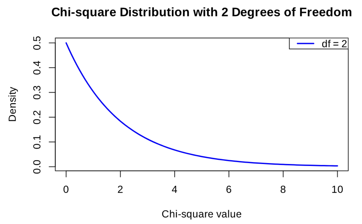
This chi-square distribution is a probability distribution. As the value of chi-square gets larger, the probability of it having been generated by the empty model will get smaller.

Calculating Chi-Square and p-Value in R

To calculate chi-square in R we can use the xchisq.test() function. Let’s try it for the current example.

xchisq.test(play_again ~ game, data=game_data)

Running this code produces this result:

  Pearson's Chi-squared test

data:  x
X-squared = 3.7915, df = 2, p-value = 0.1502

   16       11       19
(15.33)  (15.33)  (15.33)
[0.029]  [1.225]  [0.877]
< 0.17>  <-1.11>  < 0.94>

   19       24       16
(19.67)  (19.67)  (19.67)
[0.023]  [0.955]  [0.684]
<-0.15>  < 0.98>  <-0.83>

key:
  observed
  (expected)
  [contribution to X-squared]
  <Pearson residual>

Here we won’t reject the null model (that there is no effect of game) because there is a 0.15 probability of getting a frequency table like our sample if there was no effect in the DGP.