11.11 Pairwise Comparisons

It might be good enough just to know that the complex model, the one that includes game, is significantly better than the empty model. But sometimes we want to know more than that. We want to know which of the three games, specifically, are more effective in the DGP, and which just appear more effective because of sampling variation.

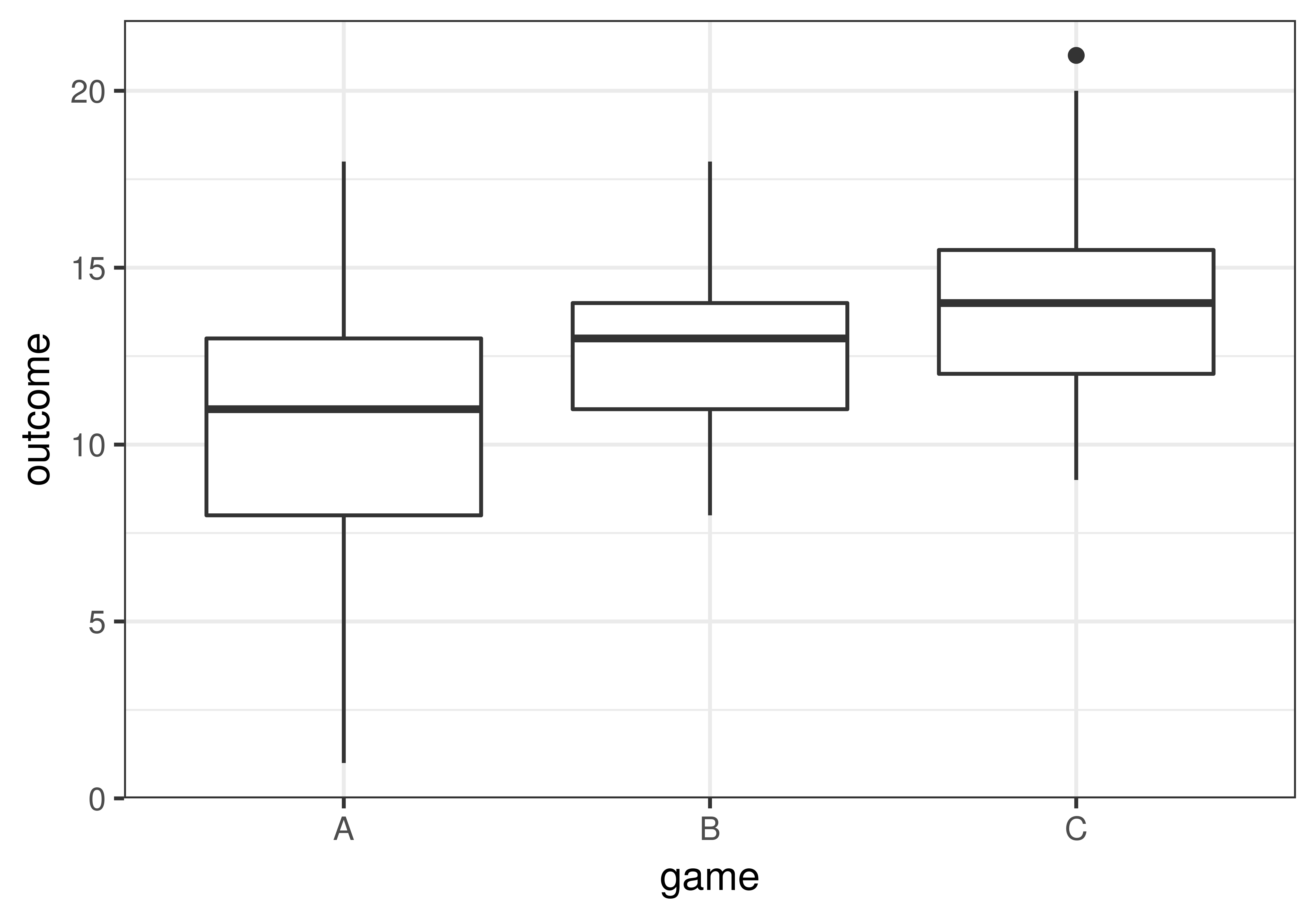
In our data (we’ve reproduced the boxplot below), it appears that game C’s students learned more than game B’s, who in turn learned more than game A’s. But such differences could be caused by sampling variation and not by real differences in the DGP. If we were to claim there is a difference in the DGP but it was actually just a difference caused by sampling variation, we would be fooled by chance (i.e., making a Type I Error).

To figure out which groups differ from each other in the DGP we can do three model comparisons, each designed to test the difference between one of the possible pairs of the three games: A vs. B, B vs. C, and A vs. C. The three model comparisons would be:

1. a model in which A and B differ to one in which they are the same (the empty model);
2. a model in which B and C differ compared to the empty model; and
3. a model in which A and C differ compared with the empty model.

The models being compared for all three pairwise comparisons would be represented the same way in GLM notation:

Model comparing two games: \(Y_i=\beta_0+\beta_1X_i+\epsilon_i\)

Versus the empty model: \(Y_i=\beta_0+\epsilon_i\)

In other words, we would be doing three separate two-group comparisons, where \(X_i\) is coded 0 or 1 depending on which of the two games are being compared. Each comparison would yield a separate F statistic, which we could interpret using the appropriate F-distribution.

The pairwise() Function

A handy way to implement these pairwise model comparisons is using the pairwise() function in the supernova R package. Previously, we saved the three-group model of game predicting outcome in an R object called game_model. We can run the code below to get the pairwise comparisons.

pairwise(game_model, correction="none")

The pairwise() function produces this output:

Model: outcome ~ game

Levels: 3

Family-wise error-rate: 0.143


  group_1 group_2  diff pooled_se     t    df lower upper p_val
  <chr>   <chr>   <dbl>     <dbl> <dbl> <int> <dbl> <dbl> <dbl>
1 B       A       2.086     0.516 4.041   102 1.229 2.942 .0001
2 C       A       3.629     0.516 7.031   102 2.772 4.485 .0000
3 C       B       1.543     0.516 2.990   102 0.686 2.400 .0035

Notice that in the pairwise table, there is a column called p_val at the end. This is the same p-value that we have been learning about: the probability of generating a statistic (in this case \(b_1\), the mean difference) more extreme than our sample if the empty model is true.

According to these individual pairwise comparisons, it seems as though all three groups are different from each other! But now that we are doing 3 “tests” of significance instead of just one overall F test of the three-group model, we have created a new problem: the problem of simultaneous inference.