12.9 Confidence Intervals and Model Comparison

We have now used the sampling distribution of \(b_1\) for two purposes: deciding whether or not to reject the empty model (or null hypothesis); and constructing a confidence interval. Now let’s think just a bit about how these two uses fit together.

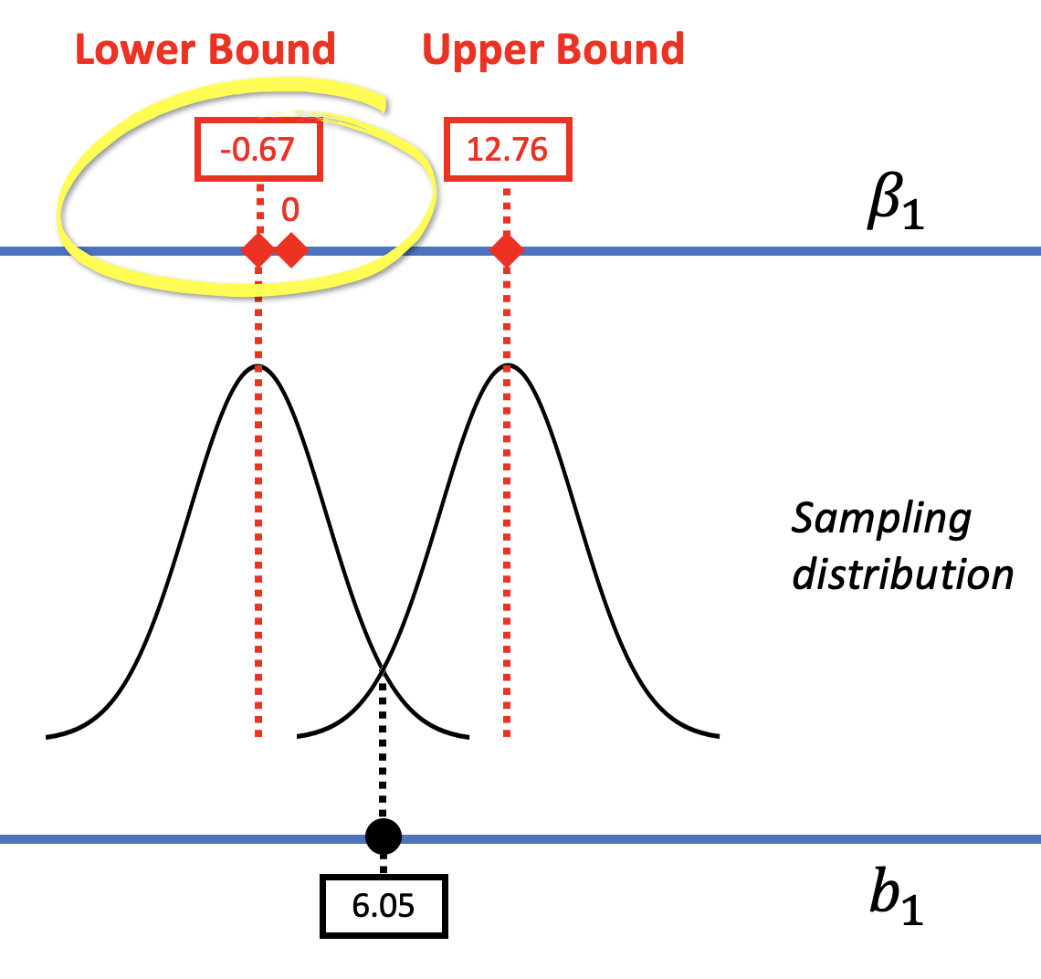
The confidence interval provides us with a range of models of the DGP (i.e., a range of possible \(\beta_1\)s) that we would not reject. In the case of the tipping study, we can be 95% confident that the true effect of smiley faces on tips in the DGP lies somewhere between -.67 and 12.76.

We would reject any values of \(\beta_1\) that do not fall within our confidence interval. In this case, 0 happens to fall within the confidence interval (see the left panel in the figure below) and so we do not rule it out as a possible model of the DGP.

Using A Confidence Interval to Evaluate the Empty Model	Using a Hypothesis Test to Evaluate the Empty Model

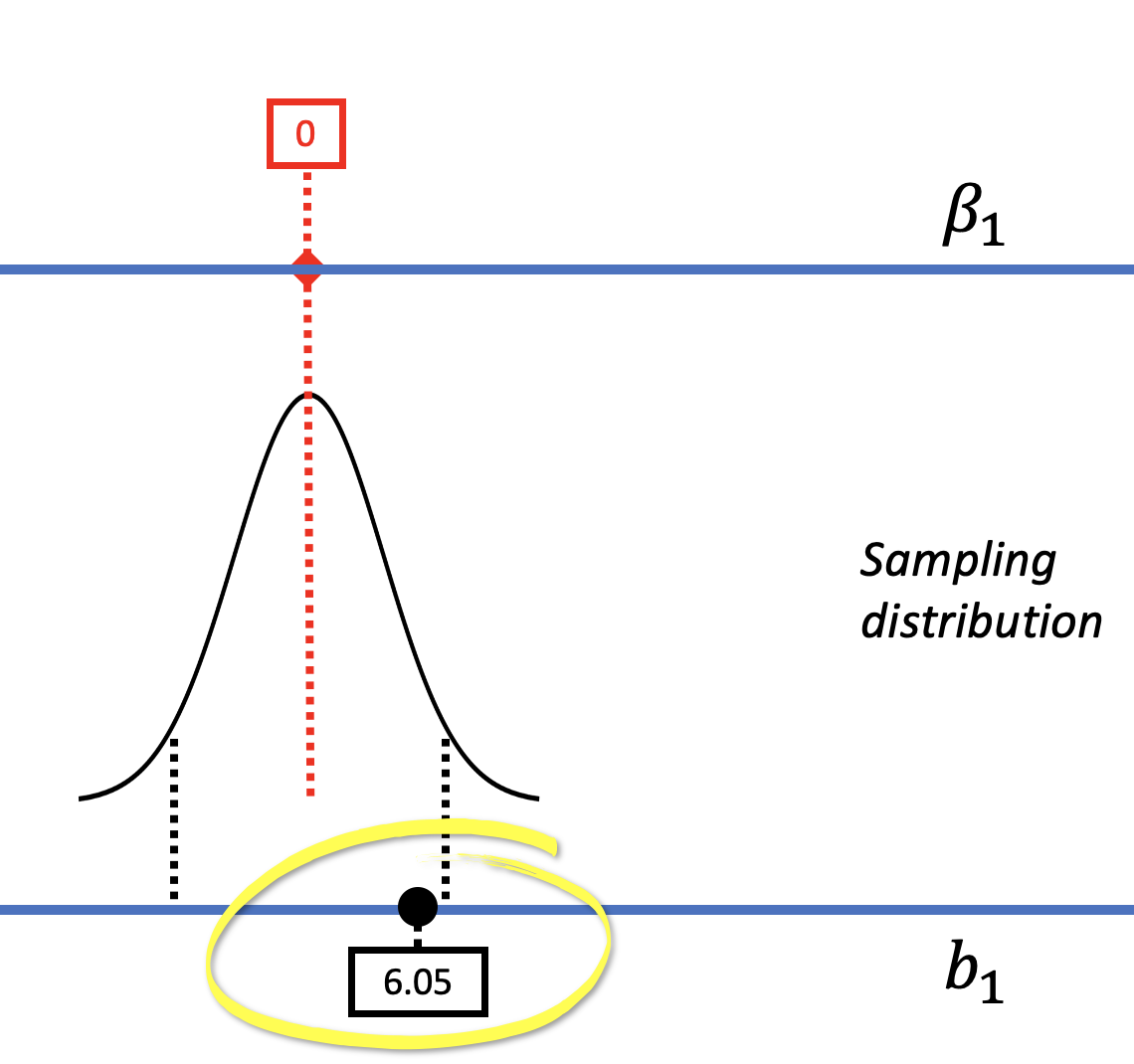
In the right panel of the figure above, the model comparison (or hypothesis testing) approach considers just one particular model of the DGP, not a range of models. In this model, in which \(\beta_1=0\) (also called the empty model or null hypothesis), there is no effect of smiley face in the DGP. We used shuffle() to mimic such a DGP, and built a sampling distribution centered at 0. We can see in the picture above that if such a DGP were true, our sample \(b_1\) would not be unlikely.

We then used the sampling distribution as a probability distribution to calculate the probability of getting a sample \(b_1\) of $6.05 or more extreme, whether positive or negative, if the empty model were true (i.e., the p-value). Based on the p-value of .08, we decided to not reject the empty model, .08 being slightly higher than the .05 cutoff we had set as our alpha criterion.

These two approaches – null hypothesis testing and confidence intervals – both provide ways of evaluating the empty model, and both lead us to the same conclusion in the tipping study: the empty model, where \(\beta_1=0\), cannot be ruled out as a possible model of the DGP.

If the 95% confidence interval does not include 0, then we would reject the empty model because we are not confident that \(\beta_1=0\). And if the confidence interval does not include 0, the p-value for the null hypothesis test would be less than .05, again leading us to reject the empty model. This is not just a coincidence. The two approaches will always corroborate each other because both are based on the same underlying logic and the same sampling distributions (i.e., with the same shape and spread).

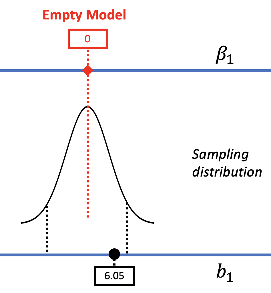
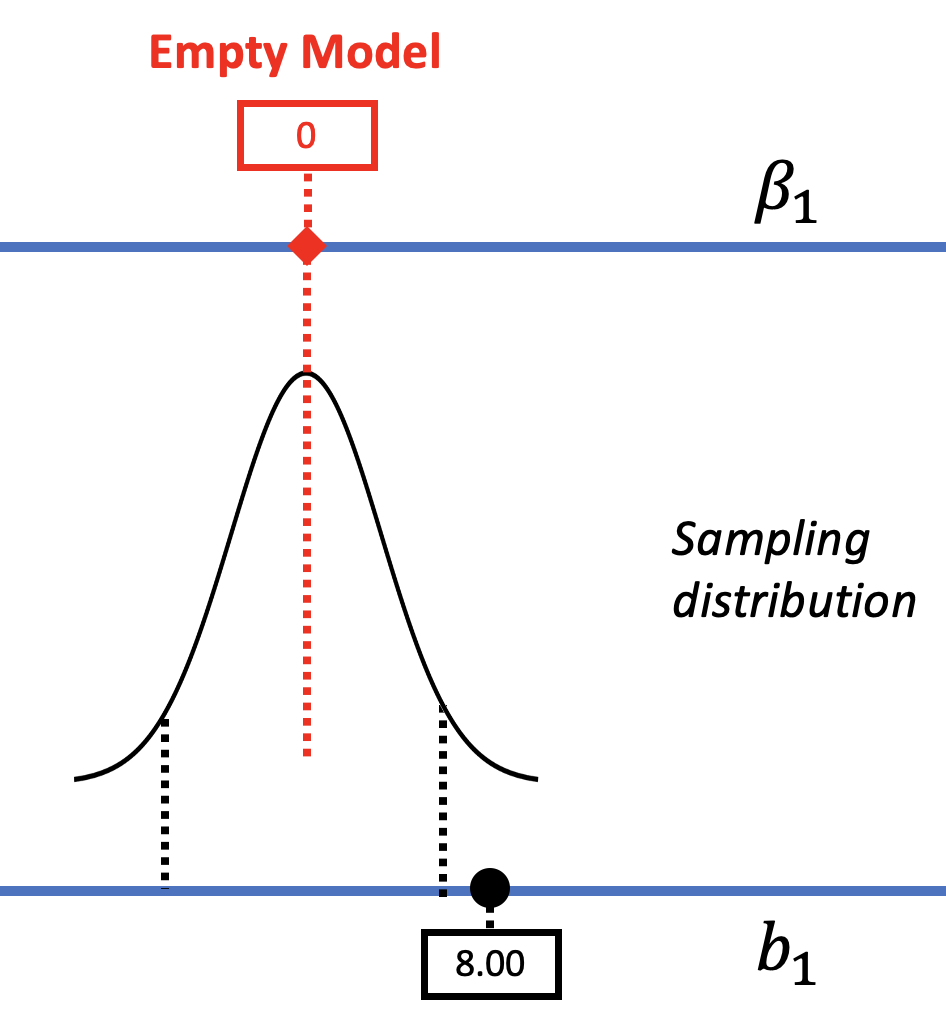
As another example, let’s consider a second tipping study done by another team of researchers. They got very similar results but this time, their \(b_1\) was $8 (see right panel of figure below), instead of $6.05 (pictured in the left panel). Their standard error (and margin of error) was the same as in the original study. The figure below represents the results of the two studies in the context of a sampling distribution from a DGP where \(\beta_1=0\).

Original Study (\(b_1=6.05\))	Second Study (\(b_1=8.00\))

We don’t really believe that the DGP has changed, so we wouldn’t say the \(\beta_1\) has changed for this study. But everything else would change – the best estimate of \(\beta_1\), the p-value, and the confidence intervals. The p-value will be lower because the \(b_1\) would now be in the unlikely tails if the empty model were true in the DGP.

Let’s take a look at how the confidence interval might be different across these two studies.

Original Study (\(b_1=6.05\))	Second Study (\(b_1=8.00\))

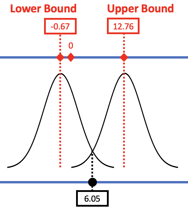
In the left panel of the figure the confidence interval (marked by the two red boxes) is centered around an assumed \(\beta_1\) that is the same as the observed \(b_1\) (6.05), and 0 is just inside the confidence interval. In this study, we did not reject the empty model as a model of the DGP because it was one of the values included in the 95% confidence about.

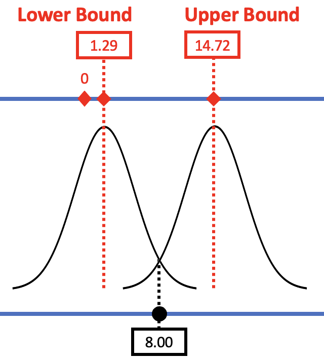
In the right panel of the figure, we see what happened in the second study where the observed \(b_1\) was a little higher (8.00). The new confidence interval is centered at 8.00, and 0 is now outside the confidence interval. Based on the results of this second study, we would reject the empty model as a model of the DGP.

It is also worth noting that we get a lot more information from the confidence interval than we do from the p-value. For example, in the original tipping study (where \(b_1 = 6.05\)), even when we don’t reject the null hypothesis (0), we would not want to therefore accept it and claim that 0 is the true value of \(\beta_1\). We can see from the confidence interval that even though the true value of \(\beta_1\) in the DGP might be 0, there are many other values it also might be. Confidence intervals help us to remember this fact.