12.8 Interpreting the Confidence Interval

Now that we have spent some time constructing confidence intervals, it is important to pause and think about what a confidence interval means, and how it fits with other concepts we have studied so far.

Confidence Intervals Are About the DGP

One common misconception about confidence intervals is that they define lower and upper cutoffs for where .95 of the \(b_1\)s might fall (see the left part in the figure below). We can forgive you if you are thinking this, because we did just spend time calculating a confidence interval by centering a sampling distribution at the sample \(b_1\), and then finding the values of \(b_1\) that would fall beyond the two .025 cutoffs.

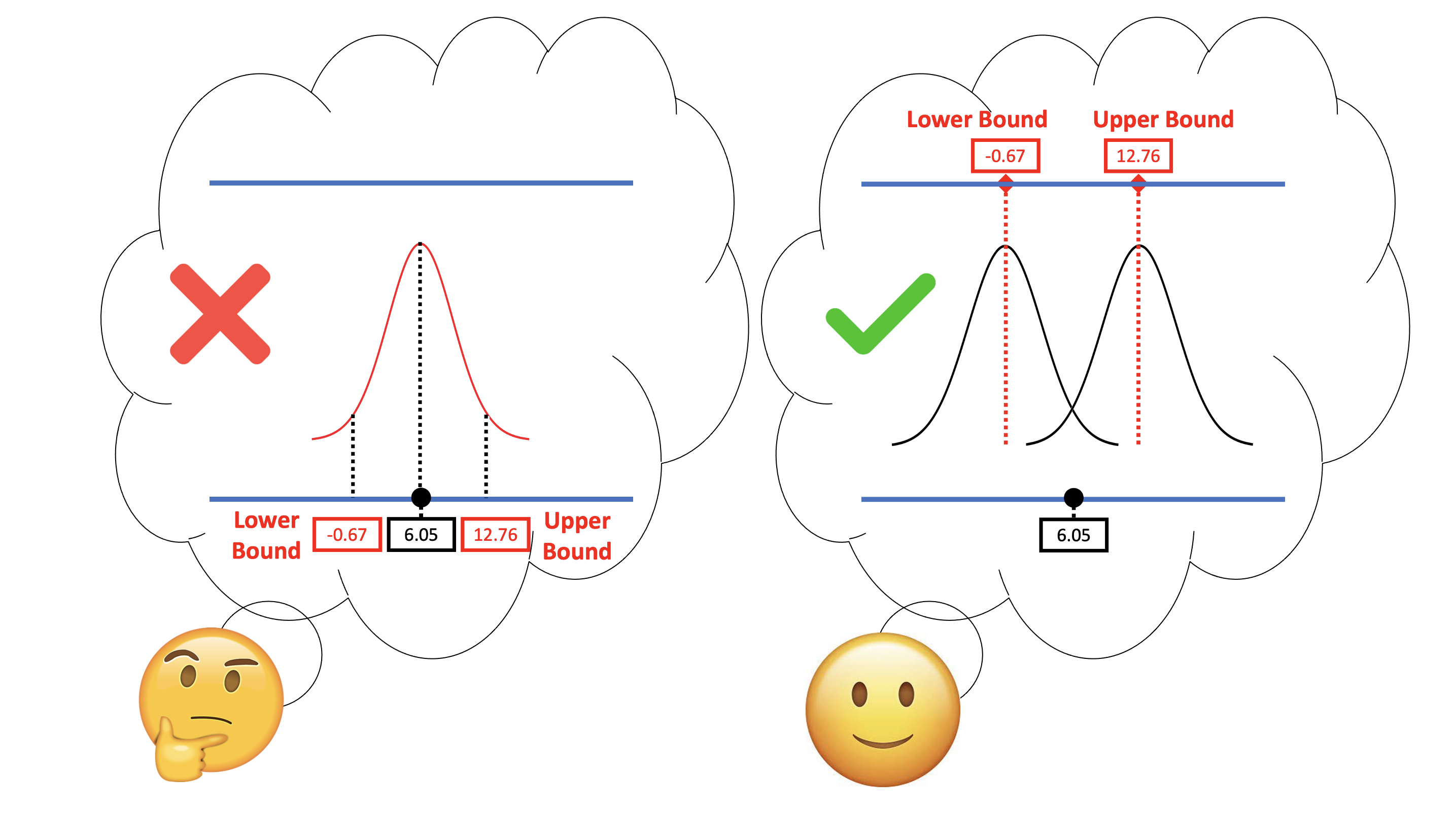
But that was just a method for calculating the interval, not a definition of what the interval actually refers to. It is important to remember that the concept of confidence interval was developed by mentally moving the sampling distribution of \(b_1\)s up and down the scale of \(\beta_1\), considering the alternative values of \(\beta_1\) in the DGP that could, with 95% likelihood, have produced the sample \(b_1\) found by the researchers. (The right part of the picture above will remind you of this way of thinking.)

If we did want to know the range of possible sample \(b_1\)s that are likely in the world, we would actually need to know the true \(\beta_1\) in the DGP. But we don’t know this. This is why we have to hypothesize lots of different values of \(\beta_1\) by sliding the sampling distribution around. Each \(\beta_1\) generates a different range of likely \(b_1\)s.

Error in an Estimate

The \(b_1\) observed by the researchers is the best estimate of what the true \(\beta_1\) might be. This estimate is often referred to as a point estimate. Based on the available data, which generally just comes from the current study, it is the best estimate the researchers can come up with for what the true \(\beta_1\) is. There is no reason to guess higher or lower than this point estimate.

But being the best doesn’t mean it’s right. This estimate is almost certainly wrong. It might be too low or it might be too high, but we don’t know which way it is wrong. And to make matters worse, it’s hard to tell whether the estimate is correct or not, or how far off it is from the true DGP, because we don’t really know what the true \(\beta_1\) is.

The confidence interval provides us with a way of addressing this problem. It tells us how wrong we could be, or put another way, how much error there might be in our estimate.

If the confidence interval is relatively wide given the situation, as it is in the tipping study, we would be saying something like, “the estimated effect of adding a smiley face to the check is $6.05. But there is a lot of error in the estimate. The true effect could be as low as 0 or slightly below that, or as high as $13.”

The width of the confidence interval (CI) tells us what the true \(\beta_1\) in the DGP might be. When the CI is narrower, we think our estimate is closer to the true \(\beta_1\) than when the CI is wider.

It is important to note that when we talk about the error in an estimate we are using the term error to mean something a little different than we have learned up to now. Previously, when we developed the concept of error (as in DATA = MODEL + ERROR), we were referring to the gap between the predicted tip for each table based on a model, and the actual tip left by that table. The errors were the individual residuals for each table.

When we think about error around a parameter estimate though, we’re not thinking about individual tables any more. A single table can’t have a \(b_1\)! A single table can’t have an average difference between control and smiley face tables. The idea of \(b_1\) only exists at the level of a whole sample. Error in \(b_1\), therefore, means how different the sample estimate is from the true \(\beta_1\) in the DGP.

Because we generally don’t know what the true \(\beta_1\) is, we can’t know how far the estimate is from the true \(\beta_1\). But because we have a sampling distribution, we can know how much the estimate might vary across samples given a particular DGP, and based on that, how much variation or error there might be in the range of possible \(\beta_1\)s that could have produced the sample estimate.

In the case of the tipping experiment, we started with a point estimate of the \(\beta_1\) parameter ($6.05) – the effect of having a smiley face on a table’s tip. The confidence interval is not telling us about the range of tips provided by all the tables in the study, but about the range of possible \(\beta_1\)s that could have generated our particular \(b_1\). In other words, it tells us how wrong our point estimate might be.

What Does the 95% Mean?

One question you might have is this: what does it mean to have 95% confidence?

Let’s start by explaining what it does not mean. It does not mean that there is a .95 probability that the true \(\beta_1\) falls within the confidence interval. This is a confusing point, and one statisticians care a lot about. If you say there’s a 95% chance that the true parameter falls in this range, they will correct you.

One reason they will correct you is that \(\beta_1\) either is in this range (100%) or is not in this range (0%). You don’t know what \(\beta_1\) is so you can’t tell if the probability is 100% or 0% but it’s definitely not a 95% probability. What is uncertain is your knowledge (measured in confidence rather than probability).

The other reason they will correct you is that there isn’t actually a .95 chance that the \(\beta_1\) is in a certain range if the sample \(b_1=6.05\), but rather a .95 chance of getting the observed sample \(b_1\) if the \(\beta_1\) is within a certain range. In probability theory, the probability of A given B is not the same as the probability of B given A, which is another way of saying the probability of B if A is true. (This is related to Bayes’ Rule, something you might want to dig deeper into, but we won’t do that here.)

Because of this issue, someone (actually, a mathematician named Jerzy Neyman, in 1937) came up with the idea of saying “95% confident” instead of “95% probable.” Our guess is that all the statisticians and mathematicians breathed a sigh of relief over this.

When you construct a 95% confidence interval, therefore, you are saying that you are 95% confident (alpha = .05) that the true \(\beta_1\) in the DGP falls within the interval. You can’t have a 100% confidence interval, by the way, because the probability model we use for the sampling distribution – the t-distribution – has tails that never really touch 0 on the y-axis. Because of this, we can’t really define the point at which the probability of Type I error would be equal to 0.