6.2 The Beauty of Sum of Squares
As it turns out, Sum of Squares (SS) has a special relationship to the mean. In the previous chapter we extolled the virtues of the mean. Now it’s time to start appreciating the beauty of sum of squares!
Sum of Squares is Minimized at the Mean
The advantage of SS as a measure of total error is that it is minimized exactly at the mean. And because our goal in statistical modeling is to reduce error as much as possible, this is a good thing.
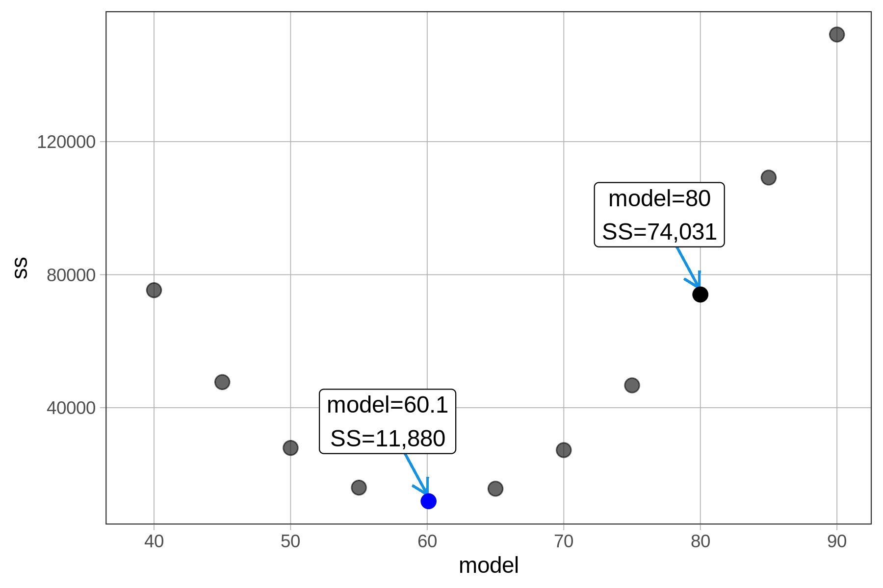
Let’s explore this idea and see if it really holds up. As a reminder, if we use the mean of 60.1 mm to predict thumb length, and then square and sum the residuals from the mean across all rows in the Fingers data set, we get 11,880.
model <- mean(Fingers$Thumb)
sum((Fingers$Thumb - model)^2)11880.2109191083By saying the sum of squares is minimized at the mean we are saying that if we calculated residuals from any number other than the mean, the sum of squares would be larger than 11880.21. Is this true?
In the code window below, we’ve set the mean of Thumb as the model prediction (model <- 60.1). Run the code and confirm that you get 11880.21 as the sum of squares.
require(coursekata)
# this sets the model at a particular value
model <- 60.1

# this calculates the sum of squares from the model
sum((Fingers$Thumb - model)^2)
# this sets the model at a particular value
model <- 60.1

# this calculates the sum of squares from the model
sum((Fingers$Thumb - model)^2)
ex() %>% check_error()Now change the model from 60.1 to 60.0 and run the code again. What happens to the sum of squares? If SS is really minimized at the mean, then it should be greater than 11,880.21 when you use any number other than the mean.
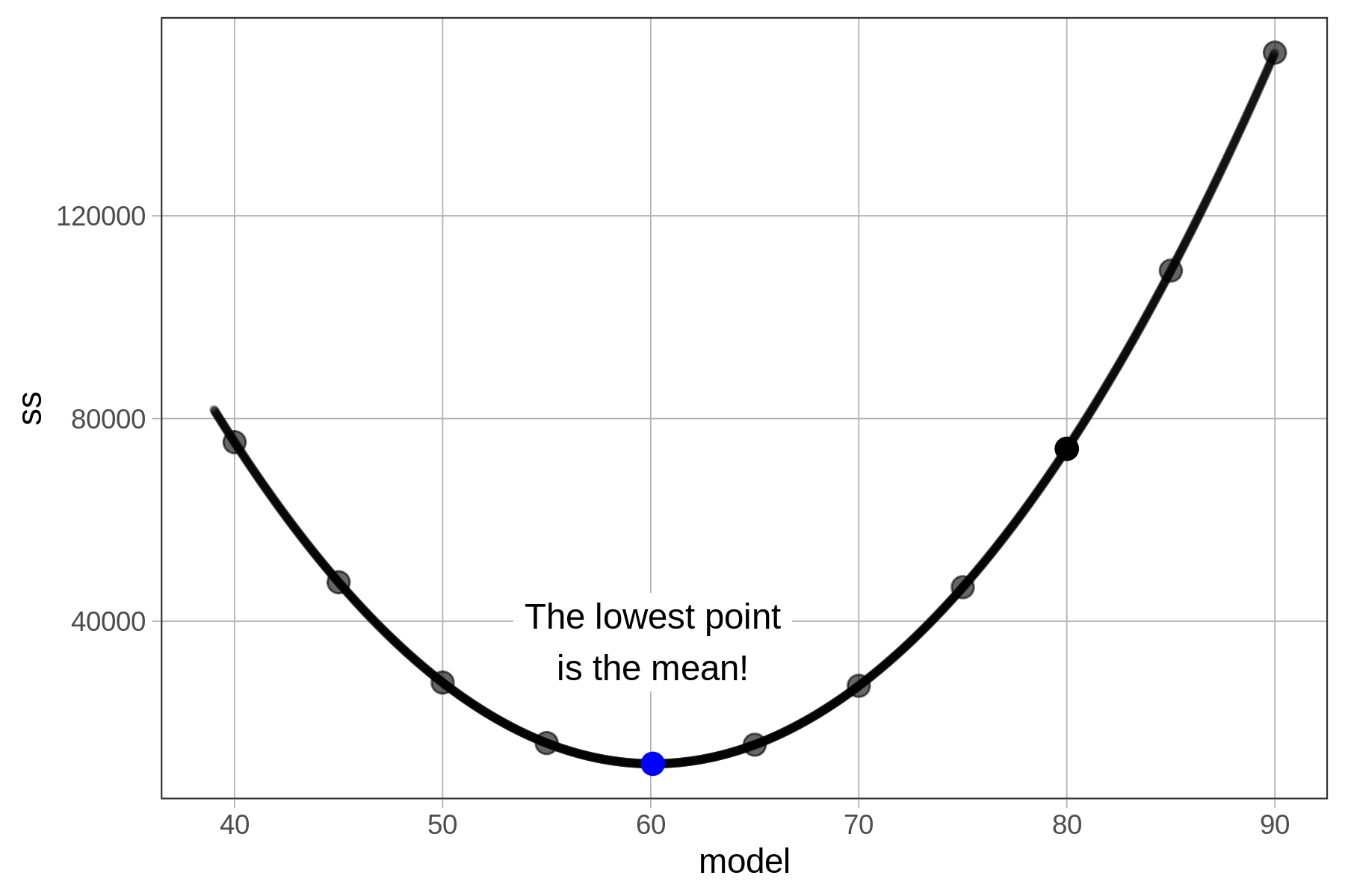
Try using some other numbers as the model and see if you can make the SS go lower! We’ve tried some ourselves and plotted them on the graph below.
When we plot the sums of squares this way they form a pattern – a kind of parabola (if you remember the shape from your algebra days). In fact, it can be proven mathematically, using calculus, that the sums of squares can never be lower for any number other than at the mean of the distribution. (A smoothed out version of the function is shown below).
The Mean and SS Go Hand-in-Hand
It is worth pointing out that the advantage of SS as an indicator of how well a model fits is only there if our model is the mean. If we were to choose another number, such as the median, to model a distribution, we would probably choose a different measure of error – presumably one that is minimized at the median. In this course we focus primarily on the mean, so we will choose SS as our preferred measure of error.
At first glance, many topics in statistics seem like part of some endless list of unrelated formulas—the mean, the sum of squares, linear models. But hopefully you are starting to see that these all fit together. The relationship between the mean and the SS is actually just one example of the interlocking relationships that connect all these concepts. The sum of squares will link up with other ideas in statistics later.
It is somewhat like the Pythagorean Theorem. You learned in school that the square of the hypotenuse of a right triangle is equal to the sum of the squares of the two sides. Thus, \(a^2+b^2=c^2\). Squaring the sides makes everything add up and fit together. But if you don’t square them, the theorem no longer holds: \(a+b\neq{c}\). By using sum of squares as a quantification of total error, lots of things will fit together that otherwise would not.
Finding Sum of Squares
Hopefully we have convinced you that SS goes hand-in-hand with the mean. More generally, we will use SS as our indication of model fit – and seek to minimize it – for all models we consider under the General Linear Model (GLM). So far, we have only explored one model – the empty model (\(Y_i=b_0+e_i\)) – in which \(b_0\) represents the sample mean (which is also our estimate of the parameter, the population mean).
As we move later to fit more complex models to data we will rely on ANOVA tables to compute the sums of squares. (ANOVA stands for ANalysis Of VAriance.) In this book we will use the supernova() function in R to produce ANOVA tables. Let’s see how it works for the empty model of Thumb.
supernova(empty_model)In the code window below, save the best-fitting empty model of Thumb as empty_model. Then try out the supernova() function, using empty_model as the input.
require(coursekata)
# create an empty model of Thumb length from Fingers
empty_model <-

# analyze the model with supernova() to get the SS
supernova()
empty_model <- lm(Thumb ~ NULL, data = Fingers)
supernova(empty_model)
ex() %>% {
    check_object(., "empty_model") %>% check_equal()
    check_output_expr(., "supernova(empty_model)")
}Analysis of Variance Table (Type III SS)
Model: Thumb ~ NULL
SS df MS F PRE p
----- ----------------- --------- --- ------ --- --- ---
Model (error reduced) | --- --- --- --- --- ---
Error (from model) | --- --- --- --- --- ---
----- ----------------- --------- --- ------ --- --- ---
Total (empty model) | 11880.211 156 76.155 As you can see, most cells in this ANOVA table are empty; we will be filling them up later as we learn how to fit more complex models. For now, we will focus on the last row, labeled Total (empty model), and the column labeled SS.
In the table, the SS for the empty model is 11880.211, the same number we got before by calculating residuals, squaring them, and then summing them across each row of the data set.