Import Data from a Google Sheet

The easiest way to import your own data into a Jupyter notebook is to first get the data in a Google Sheet, laid out in rows and columns, and then import the Google Sheet into a data frame in R. Here’s a step-by-step guide for how to do this (with an example you can try yourself):

STEP 1. Organize your data into tidy format—rows and columns.

STEP 2. Copy/Paste (or enter) your data into a Google Sheet.

As an example we’ve created a Google Sheet with the data from a study by deLoache, Miller & Rosengren (1997). (Click here to download the deLoache, Miller, and Rosengren original research article (PDF, 608KB) and here to download the deLoache, Miller, and Rosengren data (CSV, 756 bytes))

STEP 3. Make the Google Sheet public

Once you are in your own copy of the Google Sheet, click on the <Share> button in the upper right. At the bottom of the window that opens, under Get Link, click on Change to anyone with the link (see left panel of figure below). Then just click <Done> (right panel of figure).

STEP 4. Go to the File menu and select Publish to the Web.

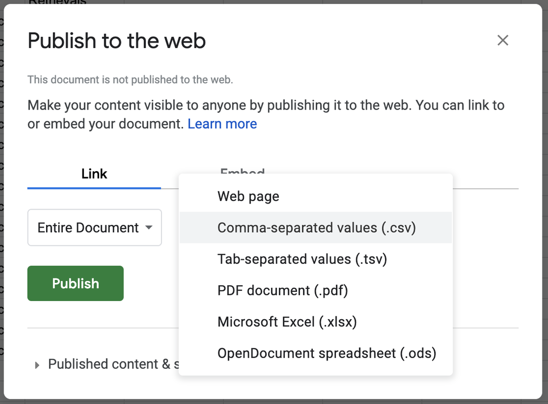
Where it says Web Page in the drop down menu, change it to Comma-separated values (.csv) (see picture). Then click the <Publish> button. This makes the data in your Google Sheet available to anyone on the internet with the link.

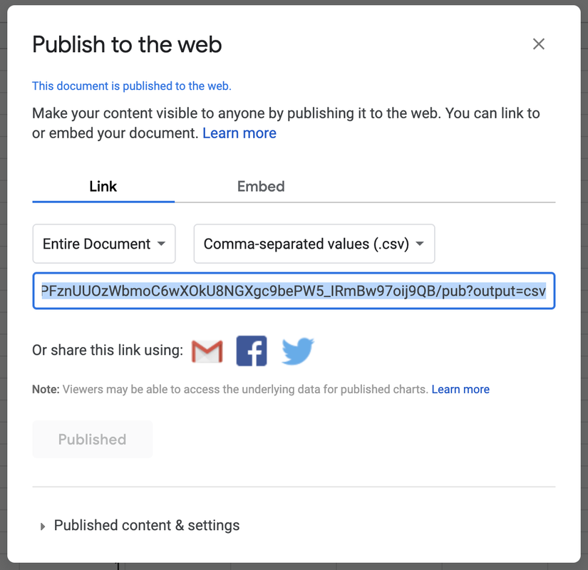
STEP 5. Copy the shareable link (highlighted in blue) to the clipboard.

STEP 6. Open your Jupyter notebook and run this code in a code block:

link <- "http://crazy_long_url_that_you_get_from_google"
example_data_frame <- read.csv(link, header=TRUE)

Be sure to replace the url between the quotes with your shareable link (keeping the quotes), and replace example_data_frame with a name of your choice.

Note: the header=TRUE argument indicates that the first row of the data file contains the variable names. If it doesn’t, simply omit this part of the code.

EXAMPLE CODE:

Continuing our example, let’s call the data frame deloache1997. Here’s some code you can paste directly into a Jupyter code cell to import the data.

require(coursekata)

# Save the link to the google sheet into an R object named csvlink
csvlink <- "https://docs.google.com/spreadsheets/d/e/2PACX-1vSb88NlGCW93VSbl4XiPaxf1iDPhbNDgG2FToX3MHxjr0-Bl4eAKQ9HlMoCW_Of0pXqLIfvP8AVb26L/pub?gid=1002384760&single=true&output=csv"

# Save the data into a data frame called deloache1997
deloache1997 <- read.csv(csvlink, header = TRUE)

# check out the contents of the new data frame
str(deloache1997)

You should get the output below, showing 32 observations and four variables: Age, Gender, Condition, Retrievals.

'data_frame' :  32 obs. of  4 variables:
 $ Age       : int  29 29 29 30 30 30 31 31 31 31 ...
 $ Gender    : Factor w/ 2 levels "female","male": 1 2 1 2 1 2 1 1 2 1 ...
 $ Condition : Factor w/ 2 levels "Nonsymbolic",..: 1 1 1 1 1 1 1 1 1 1 ...
 $ Retrievals: int  4 3 2 4 3 2 4 4 3 2 ...