5.5 Fitting the Empty Model

The simple model we have started with—using the mean to model the distribution of a quantitative variable—is sometimes called the empty model or null model. In the context of students’ thumb lengths, we could write the empty model with a word equation like this.

Thumb = Mean + Error

Note that the model is “empty” because it doesn’t have any explanatory variables in it yet. The empty model does not explain any variation; it merely reveals the variation in the outcome variable (the Error) that could be explained. This empty model will serve as a sort of baseline model to which we can compare more complex models in the future.

If the mean is our model, then fitting the model to data simply means calculating the mean of the distribution, which we could do using favstats().

favstats(~ Thumb, data = Fingers)

min Q1 median Q3 max     mean       sd   n missing
  39 55     60 65  90 60.10366 8.726695 157       0

When we fit a model we are finding the particular number that minimizes error the most; this is what we mean by the “best-fitting” model. The mean of a distribution is one such number because it balances the residuals. In later chapters, we will expand more on why this value is the best-fitting one.

It’s easy to fit the empty model—it’s just the mean (60.1 in this case). But later you will learn to fit more complex models to your data. We are going to teach you a way to fit models in R that you can use now for fitting the empty model, but that will also work later for fitting more complex models.

The R function we are going to use is lm(), which stands for “linear model.” (We’ll say more about why it’s called that in a later chapter.) Here’s the code we use to fit the empty model, followed by the output.

lm(Thumb ~ NULL, data = Fingers)

Call:
lm(formula = Thumb ~ NULL, data = Fingers)

Coefficients:
(Intercept)  
       60.1 

Although the output seems a little strange, with words like “Coefficients” and “Intercept,” the lm() function does give you back the mean of the distribution (60.1), as expected. lm() thus “fits” the empty model in that it finds the best-fitting number for our model. The word “NULL” is another word for “empty” (as in “empty model.”)

It will be helpful to save the results of this model fit in an R object. Here’s code that uses lm() to fit the empty model, then saves the results in an R object called empty_model:

empty_model <- lm(Thumb ~ NULL, data = Fingers)

If you want to see the contents of the model, you can just type the name of the R object where you saved it (i.e., just type empty_model). Try it in the code block below.

When we save the result of lm() as empty_model we are saving a new type of R object called a model, which is different from data frames or vectors. When R saves a model it saves all sorts of information inside the object, which we won’t get into here. But some functions we will learn about specifically take models as their input.

One such function is gf_model(), which lets us overlay a model (e.g., empty_model) onto various types of plots, including histograms, boxplots, jitter plots, and scatterplots.

For example, here is how to chain the empty_model predictions (using the pipe operator, %>%) onto a histogram of thumb lengths.

gf_histogram(~ Thumb, data = Fingers) %>%
gf_model(empty_model)

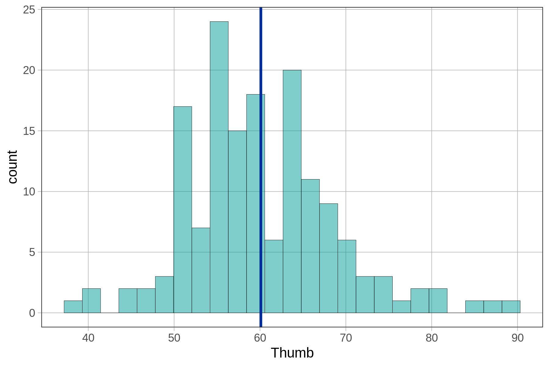
As we now know, the empty model predicts the mean thumb length for everyone. This model prediction is represented by the single blue vertical line right at the average thumb length of 60.1 mm. Let’s try adding gf_model(empty_model) to some other plots below.

Try running the code block below and take a look at the resulting graphs. Then use the pipe operator (%>%) to add the empty model prediction to both the scatterplot of thumb lengths by height and the jitter plot of thumb lengths by sex. (The empty model has already been fit and saved as empty_model.)

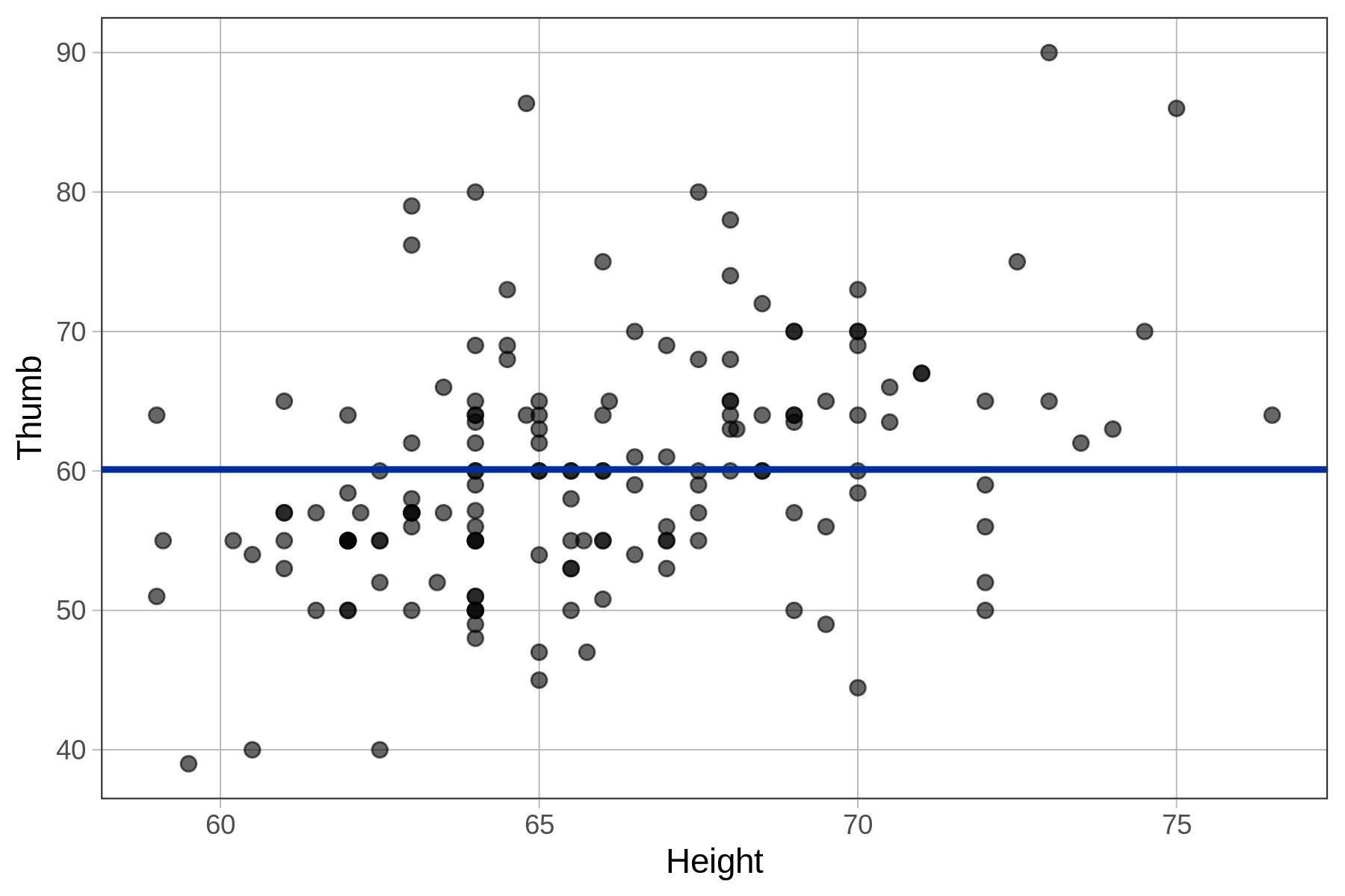
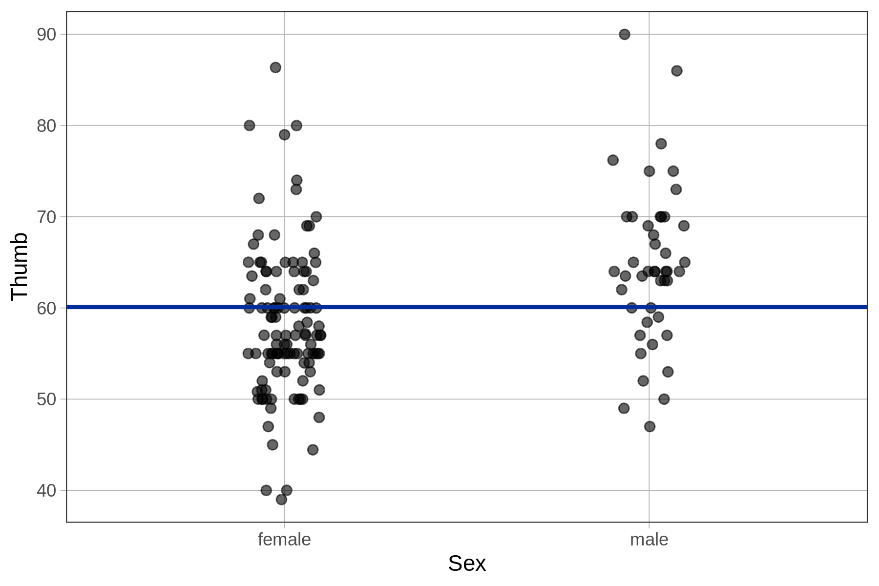
When we overlaid the empty model prediction on the histogram of Thumb, it was represented as a vertical line because Thumb was on the x-axis. With the scatterplot and jitter plot above, Thumb is on the y-axis. For this reason, the empty model prediction (i.e., the mean of Thumb) is represented as a horizontal line, right at the mean of Thumb.

The empty model prediction on the scatterplot (on the left, above), as represented by the horizontal line, indicates that regardless of how tall a student is, the empty model will assign them a predicted thumb length of 60.1 mm.

The Mean as an Estimate

We seem to be making a big deal about having calculated the mean! But trust us, it will make more sense once you see where we go with it. One point worth making now, however, is that the goal of statistics is to understand the Data Generating Process (DGP). The mean of the data distribution is an estimate of the mean of the population that results from the DGP, which is why the numbers generated by lm() are called “estimates” (or sometimes, “coefficients”).

The mean may not be a very good estimate—after all, it is only based on a small amount of data—but it’s the best one we can come up with based on the available data. The mean also is considered an unbiased estimate, meaning that it is just as likely to be too high as it is too low.