8.6 Using Shuffle to Compare Models of the DGP

Simulating the Empty Model with shuffle()

If there was truly no effect of drawing smiley faces on tips, then the empty model in which \(\beta_1 =0\) would be a good model of the DGP. But even if this were the true DGP, we would not expect our sample \(b_1\) to be exactly 0. Especially if the sample were small, it might be a little higher or a little lower than 0. The question is, how much higher or lower would it be?

We can use the shuffle() to investigate this question. But now that you have learned to fit a model, we can take shuffling to a new level. Instead of shuffling the tips and looking at the resulting plots of the shuffled groups, we can fit a model to the shuffled data and calculate an estimate of \(\beta_1\) from each shuffled sample.

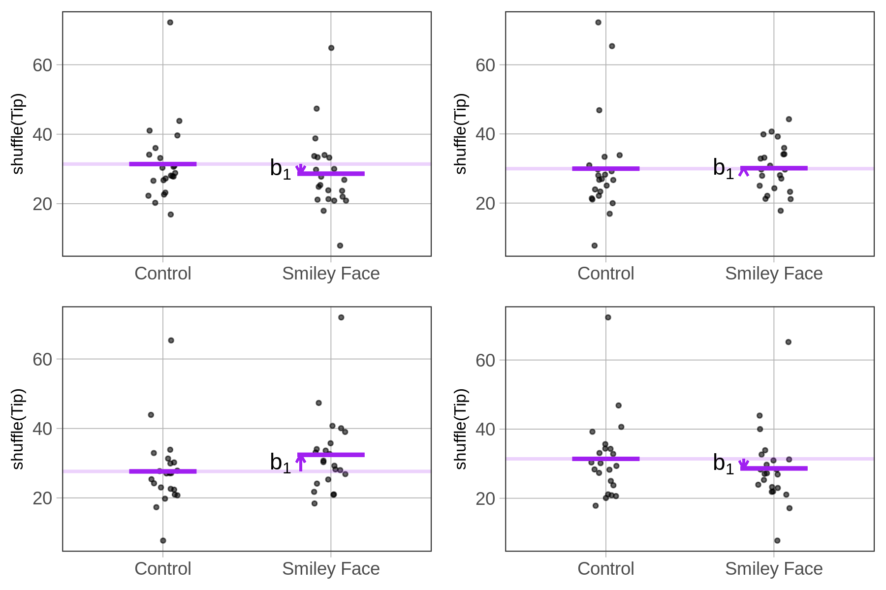
In fact, we don’t even need the graphs. We can combine the b1() function with shuffle() to directly calculate the \(b_1\) estimate for each shuffled sample. If we do this multiple times, we can look at the range of \(b_1\) estimates that are produced when the empty model is true in the DGP, and any group differences are due only to randomness.

In the code window below we’ve put code to directly calculate the \(b_1\) estimate from the tipping experiment. We’ve also put some code to shuffle the tips, and then produce the \(b_1\) estimate again based on the shuffled data. Run the code a few times and see what you get.

6.045
0.036

We got these two results when we ran the code. The 6.045 is familiar: it’s the \(b_1\) estimate we got earlier from fitting the model to the actual data using lm(). The 0.036 is what we got as the \(b_1\) estimate for shuffled data.

Because shuffling is a random process, we will get a different \(b_1\) estimate each time we run the code. Run it a few times to see what you get.

If you add the do() function in front of the code above it will repeat this random process a specified number of times, generating a new \(b_1\) each time. To get 5 shuffles, for example, you would write:

do( 5 ) * b1(shuffle(Tip) ~ Condition, data = TipExperiment)

Try modifying the code in the window below to produce 10 shuffles of the tips across conditions, and 10 randomized estimates of \(\beta_1\).

           b1
1  -3.7727273
2  -2.6818182
3  -1.4090909
4  -2.6818182
5  -4.6818182
6   2.0454545
7  -0.1363636
8  -1.1363636
9   0.5909091
10  4.6818182

The ten \(b_1\) estimates that resulted when you ran the code will not be exactly the same as the estimates we got (shown above). But notice that some of these shuffled \(b_1\)s are positive and some are negative, some are quite different from 0 (e.g., 4.68 and -3.77) and some are fairly close to 0 (e.g., -0.13). Feel free to run the code a few times to get a sense of how these \(b_1\)s can vary.

If we continue to generate random \(b_1\)s, we would start to see that although they are rarely exactly 0, they are clustered around 0. This is because shuffle simulates a DGP in which there is no effect of smiley face on tips, and in which the tables would have tipped the same amount even if they were put into the other condition.

Bear in mind: Each of these \(b_1\)s results from a random process that has nothing to do with whether the table actually got smiley faces or not. The shuffle() function mimics a DGP where \(\beta_1=0\). Sometimes the DGP is called “the parent population” because when it generates \(b_1\)s, these “children” tend to resemble their parent.

Using Simulated \(b_1\)s to Help Us Understand the Data Better

We can use these simulated \(b_1\)s to help us understand the data better. We can start with the actual \(b_1\) that resulted from the study (6.045), and then compare it to the 10 \(b_1\)s we generated based on shuffled data.

Here they are again, but this time we’ve arranged them in order from low to high.

           b1
1  -3.7727273
2  -3.2272727
3  -1.6818182
4  -1.6818182
5  -1.5000000
6  -0.5000000
7   0.1363636
8   2.7727273
9   3.6818182
10  6.9545455

What we can see now, much more clearly than when we had only the graphs to go on, is that only one of the 10 randomly generated \(b_1\)s is as high or higher than the one observed in the study. From this we might conclude that there is only a 1 in 10 chance (roughly) that we would have observed a \(b_1\) of 6.045 if the empty model is true of the DGP.

Based on this, would we want to rule out the empty model as being the true model of the DGP? That’s a hard call, and one we will return to in Chapter 9. For now, just note that seeing the observed \(b_1\) in the context of other \(b_1\)s that could have been generated from the empty model, helps us to think more critically about how we should interpret the results of the tipping study.