Chapter 6 - Quantifying Error

6.1 Quantifying Total Error Around a Model

Up to now we have developed the idea that a statistical model can be thought of as a number—a predicted value for the outcome variable. We are trying to model the Data Generating Process (DGP). But because we can’t see the DGP directly, we fit a model to our data, estimating the parameters.

Using the DATA = MODEL + ERROR framework, we have defined error as the residual that is leftover after we take out the model. In the case of our simple model for a quantitative outcome variable, the model is the mean, and the error— or residual—is the deviation of each score above or below the mean.

We represent the empty model like this using the notation of the General Linear Model:

\[Y_i=b_0+e_i\]

This equation represents each score in our data as the sum of two components: the mean of the distribution (represented by \(b_0\)), and the deviation of the score above or below the mean (represented as \(e_i\)). In other words, DATA = MODEL + ERROR.

In this chapter, we will dig deeper into the ERROR part of our DATA = MODEL + ERROR framework. In particular, we will develop methods for quantifying the total amount of error around a model, and for modeling the distribution of error itself.

Quantifying the total amount of error will help us compare models to see which one explains more variation. Modeling the distribution of error will help us to make more detailed predictions about future observations and more precise statements about the DGP.

At the outset, it is worth remembering what the whole statistical enterprise is about: explaining variation. Once we have created a model, we can think about explaining variation in a new way, as reducing error around the model predictions.

We have noted before that the mean is a better model of a quantitative outcome variable when the spread of the distribution is smaller than when it is larger. When the spread is smaller, the residuals from the model are smaller. Quantifying the total error around a model will help us to know how good our models are, and which models are better than others.

Adding Up the Residuals

The histograms below show the distribution of Thumb and the distribution of Resid for our data set. As explained earlier, these distributions have the exact same shape, but different means.

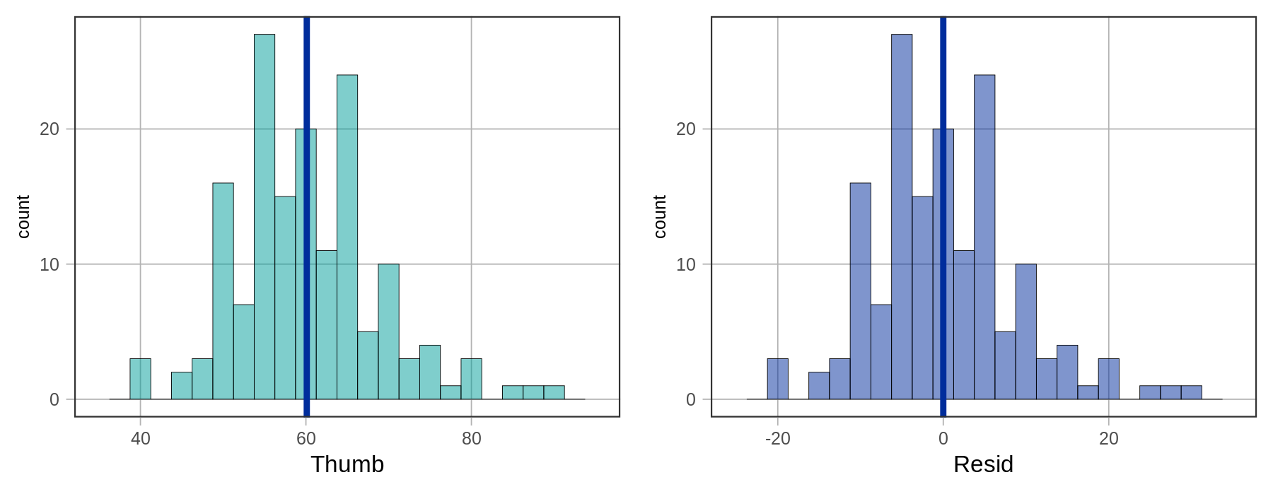
It makes sense to use residuals to analyze error from the model. If we want to quantify total error, why not just add up all the residuals? Worse models should have more error, so the sum of all the errors should represent the “total” error. The problem with this approach, as discussed previously, is that the sum of the residuals around the mean will be 0. The following code will add up all the residuals from our empty_model.

sum(resid(empty_model))

2.09277040141842e-14

Statisticians have explored various methods for quantifying error around a mean. Two of the most common, which we will discuss here are Sum of Absolute Deviations (SAD), and Sum of Squared Deviations (SS). Let’s take a look at each.

Sum of Absolute Deviations (SAD)

Sum of absolute deviations gets around the problem that deviations around the mean always add up to 0 by taking the absolute value of the deviations before summing them. We can represent this summary measure like this:

\[\sum_{i=1}^n |Y_i-\bar{Y}|\]

In this context, “deviations from the mean” means the same thing as “residuals from the empty model,” given that the mean is our model. We already have the deviations of each thumb length from the mean in the Resid column of Fingers .

We can take the absolute value of each deviation from the mean by using the function abs().

abs(Fingers$Resid)

This would print out the absolute value of all the residuals (157 of them). To get the sum, we can wrap the function sum() around abs(Fingers$Resid). Try it in the code block below.

1052.43656050955

Sum of Squared Deviations (SS)

Another way to quantify total error is to square the deviations (i.e., residuals) and then sum them. (Because squaring will result in a positive number no matter the starting value, it is not necessary to take the absolute value.) This approach can be represented like this.

\[\sum_{i=1}^n (Y_i-\bar{Y})^2\]

We already have calculated the residuals and saved them as a column called Resid. To square the residuals we can use the R code below. (Note that in R we use the caret symbol ^ to represent exponents, usually found above the 6 on a standard keyboard.)

Fingers$Resid^2

Running this code will produce a list of 157 squared residuals. Modify the code in the window below using sum() to get the sum of the squared residuals .

11880.2109191083

If you use the length of a residual to create a square (as illustrated in the figure below), the area of this square represents the size of the squared residual. Whereas thumb lengths in the Fingers data are measured in millimeters, the squared residuals are measured in square millimeters.

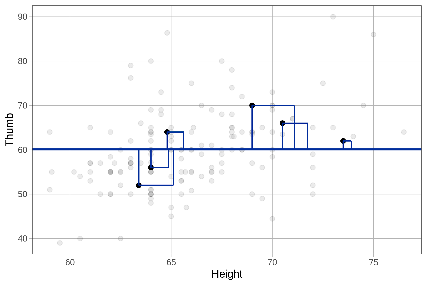
We can imagine the Sum of Squares (SS) as the total area of the squares for all the residuals in the data set. Sum of Squares will be an important indicator of how much error there is around a model’s predictions.