11.7 Using F to Compare Multiple Groups
Up to now we have used both the sampling distribution of \(b_1\) and the sampling distribution of F to compare a complex model of the DGP (either a two-group model or a regression model) to the empty model. Both approaches give similar results, resulting in a p-value that indicates the likelihood of the sample \(b_1\) or sample F being generated if the empty model is true.
Where the F-distribution really shines, however, is in comparing more complex models (i.e., ones with more parameters being estimated) with the empty model. Let’s take, for example, a three-group model, which we could represent like this:
\[Y_i = \beta_0 + \beta_1X_{1i} + \beta_2X_{2i} + \epsilon_i\]
Now we have two parameters beyond the empty model: \(\beta_1\) and \(\beta_2\). \(\beta_1\) is the increment from the first group to the second group, while \(\beta_2\) is the increment from the first group to the third group. We could, theoretically, calculate a p-value for each of the parameter estimates (\(b_1\) and \(b_2\)), but these p-values would be hard to interpret. What if one were low and the other one high? What would this say about the overall model?
The F ratio, and its corresponding sampling distribution, provides an elegant solution to this problem. Instead of having to consider \(b_1\) or \(b_2\) separately, the F statistic compares the whole complex model to the empty model. But this will subtly change how we interpret the results of the F-test. Let’s see this in action by using the F-test with a three-group model.
A Study Comparing the Effectiveness of Three Math Games
The game_data data frame contains the results of a small study comparing the effectiveness of three different computer-based math games in a sample of 105 fifth-grade students. All three games focused on the same topic and had identical learning goals, and none of the students had any prior knowledge of the topic.
Students each were randomly assigned to play one of the three math games, which we will call A, B, and C. Each student played their assigned game for a total of 10 hours spread out over a single week. At the end of the week, their learning was assessed using a common 30-item test. The research question was: Were some games more effective than others? Did the three games produce different amounts of student learning?
The game_data data frame includes 105 students and two variables:
game– the game the student was randomly assigned to, coded as A, B, or Coutcome– each student’s score on the outcome test
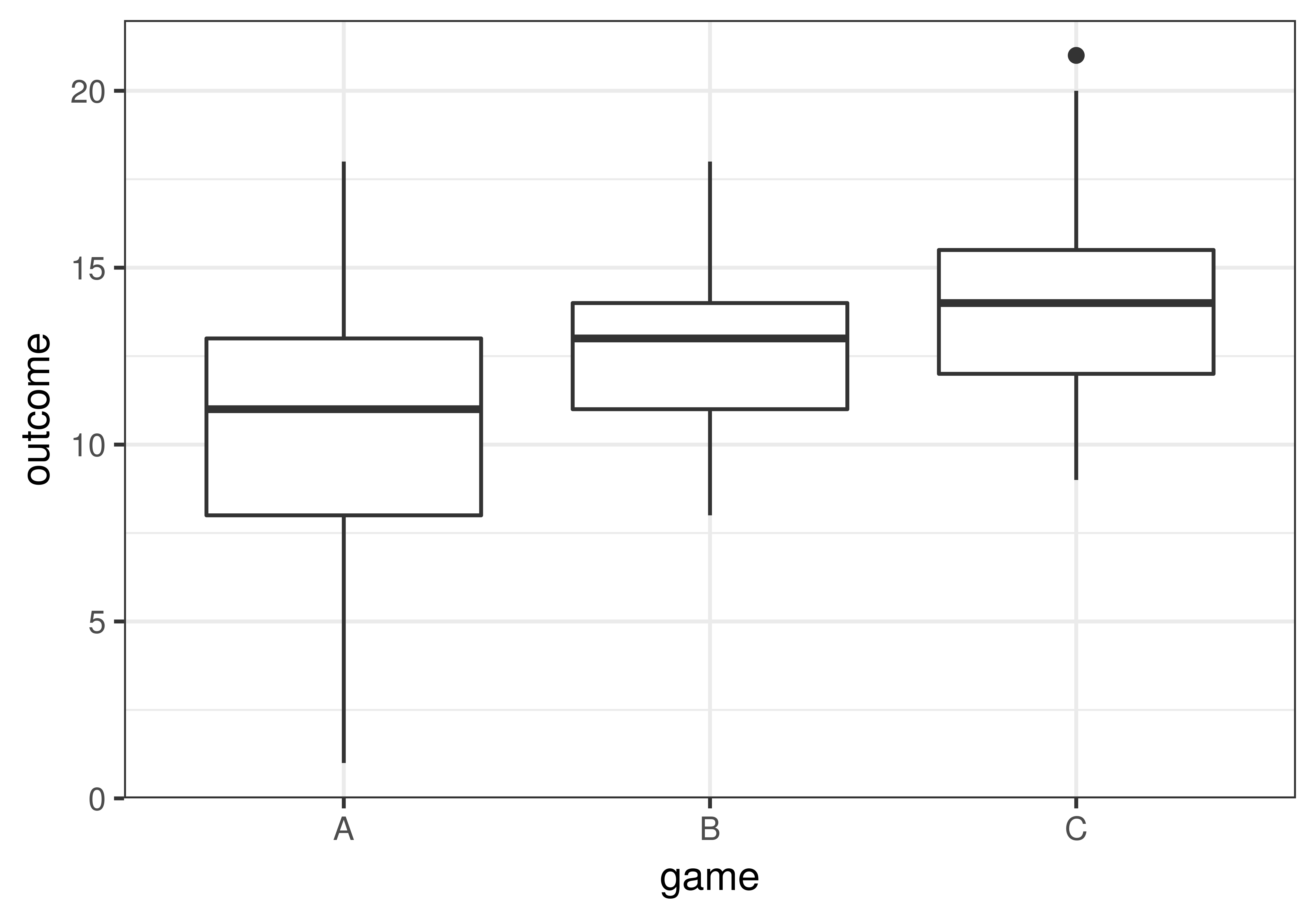
Let’s compare the variable outcome across the three games, using both gf_boxplot() and favstats().
gf_boxplot(outcome ~ game, data = game_data)
favstats(outcome ~ game, data = game_data) game min Q1 median Q3 max mean sd n missing
1 A 1 8 11 13.0 18 10.48571 3.641036 35 0
2 B 8 11 13 14.0 18 12.57143 2.512155 35 0
3 C 9 12 14 15.5 21 14.11429 2.897985 35 0It appears from both the favstats and the boxplots that game C’s students generally learned the most and game A’s students the least. Game B’s students fell in between the other two groups. It also looks like the outcomes of students who played game A varied more than students in the other two groups.
Although it appears from the boxplot that game C’s students learned more than game A’s, this does not necessarily mean that game C is more effective in the DGP. It is possible that the difference could simply be the result of random sampling variation: Maybe game C just happened to end up with a more capable group of students.
By now, you know how to re-cast this question in terms of model comparison. Which model do we want to adopt as our best guess about the DGP? The empty model, in which all three games are equally effective, or the three-group model in which the three games are not equally effective? Here are the two models in GLM notation:
The game model: \(Y_i=\beta_0+\beta_1X_{1i}+\beta_2X_{2i}+\epsilon_i\)
The empty model: \(Y_i=\beta_0+\epsilon_i\)
Fit the game model in the code window below.
require(coursekata)

# import game_data
students_per_game <- 35
game_data <- data.frame(
    outcome = c(16,8,9,9,7,14,5,7,11,15,11,9,13,14,11,11,12,14,11,6,13,13,9,12,8,6,15,10,10,8,7,1,16,18,8,11,13,9,8,14,11,9,13,10,18,12,12,13,16,16,13,13,9,14,16,12,16,11,10,16,14,13,14,15,12,14,8,12,10,13,17,20,14,13,15,17,14,15,14,12,13,12,17,12,12,9,11,19,10,15,14,10,10,21,13,13,13,13,17,14,14,14,16,12,19),
    game = c(rep("A", students_per_game), rep("B", students_per_game), rep("C", students_per_game))
)
# fit and print the game model of outcome
# fit and print the game model of outcome
lm(outcome ~ game, data = game_data)
ex() %>%
    check_function("lm") %>%
    check_result() %>%
check_equal()Call:
lm(formula = outcome ~ game, data = game_data)
Coefficients:
(Intercept) gameB gameC
10.486 2.086 3.629 In the next code window, run the supernova() function on the game_model to look at how it compares with the empty model.
require(coursekata)

# import game_data
students_per_game <- 35
game_data <- data.frame(
    outcome = c(16,8,9,9,7,14,5,7,11,15,11,9,13,14,11,11,12,14,11,6,13,13,9,12,8,6,15,10,10,8,7,1,16,18,8,11,13,9,8,14,11,9,13,10,18,12,12,13,16,16,13,13,9,14,16,12,16,11,10,16,14,13,14,15,12,14,8,12,10,13,17,20,14,13,15,17,14,15,14,12,13,12,17,12,12,9,11,19,10,15,14,10,10,21,13,13,13,13,17,14,14,14,16,12,19),
    game = c(rep("A", students_per_game), rep("B", students_per_game), rep("C", students_per_game))
)
# this code fits the game model and saves it as game_model
game_model <- lm(outcome ~ game, data = game_data)

# print the ANOVA table that compares game_model to the empty model
# this code fits the game model and saves it as game_model
game_model <- lm(outcome ~ game, data = game_data)

# print the ANOVA table that compares game_model to the empty model
supernova(game_model)
ex() %>%
    check_function("supernova") %>%
    check_result() %>%
check_equal()Using the Sampling Distribution of F to Compare the Two Models
We can see from the ANOVA table that the game model so efficiently makes use of the additional parameter estimates that the variation explained by the complex model is over 12 times bigger than the variation unexplained. But does a high F provide enough justification to reject the empty model as a model of the DGP in favor of the game model?
To reject the empty model, we want to know the probability that an F statistic as extreme as the observed F (12.45) could have been produced by the empty model, what we have been calling the p-value. If the probability is low (e.g., less than .05), then we could reject the empty model in favor of the more complex model (i.e., the game model). This is what is meant by “rejecting the null hypothesis.”
Under the empty model, the true difference between the 3 groups is equal to 0. In other words, the three games are equally effective.
To calculate the p-value , we need to create a sampling distribution of F from the empty model of the DGP. We can use randomization (e.g., shuffle()) but we can also use the F-distribution. We hope to have convinced you by now that both would lead to roughly similar outcomes. Let’s just take the latter option and use the F-distribution (which is what supernova() uses to calculate the p-value.
Analysis of Variance Table (Type III SS)
Model: outcome ~ game

                              SS  df      MS      F    PRE     p
----- --------------- | -------- --- ------- ------ ------ -----
Model (error reduced) |  232.133   2 116.067 12.451 0.1962 .0000
Error (from model)    |  950.857 102   9.322
----- --------------- | -------- --- ------- ------ ------ -----
Total (empty model)   | 1182.990 104  11.375
The p-value of .0000 represents a very, very low probability (p < .0001) of having observed an F greater than our sample F (12.45) if there were no difference in effectiveness between the games. Note that “no true difference between the three groups” also means that between all pairs of games, the true difference would be 0. Based on this result, we would reject the empty model and adopt the more complex model in which the true difference across games in their effectiveness is not equal to 0.
Interpretation of the Multi-Group F Test
A low p-value (e.g., one less than .05 or .01), which is always associated with a high F ratio, means that the probability of our data being generated by the empty model is very low, and so we would reject the empty model.
Ruling out the empty model does not mean that our alternative model (the model that best fits our data) is true. Our complex model is just one of the possible models that are consistent with our data.
In the case of a two-group model, like the one we used to compare tips between the smiley face and control groups, the interpretation of a low p-value would have been straightforward: the observed difference between the two groups is unlikely to have resulted from a world in which the true difference between the groups (in the DGP) is equal to 0. This is what we mean when we say that the difference between two groups is statistically significant. We think the difference is real in the DGP.
With a three-group model, however, the interpretation of a low p-value is a little more complicated. It means that we can be confident that the empty model (where the three groups are equal to each other) is not a good model of the DGP that produced our sample and that the game model is significantly better. The low p-value tells us that the three games have a less than .05 chance of producing the same amount of learning in the DGP.
Rejecting the empty model does not tell us, however, which of the three games differ significantly from each other and which might not differ. The overall F test allows us only to compare the complex model as a whole to the empty model. If we want to know which games differed from which other games we will need a new technique: pairwise comparisons.