7.10 Using Proportional Reduction in Error (PRE) to Compare Two Models
We have now quantified how much variation has been explained by our model: 1,334 square millimeters. But is that a lot of explained variation, or just a little? It would be easier to understand if we knew the proportion of total error that has been reduced rather than the raw amount of error reduced measured in \(mm^2\).
If you take another look at the supernova() table (reproduced below) for the Sex_model, you will see a column labeled PRE. PRE stands for Proportional Reduction in Error.
Analysis of Variance Table (Type III SS)
Model: Thumb ~ Sex

                               SS  df       MS      F    PRE     p
----- --------------- | --------- --- -------- ------ ------ -----
Model (error reduced) |  1334.203   1 1334.203 19.609 0.1123 .0000
Error (from model)    | 10546.008 155   68.039
----- --------------- | --------- --- -------- ------ ------ -----
Total (empty model)   | 11880.211 156   76.155
PRE is calculated using the sums of squares. It is simply SS Model (i.e., the sum of squares reduced by the model) divided by SS Total (or, the total sum of squares in the outcome variable under the empty model). We can represent this in a formula:
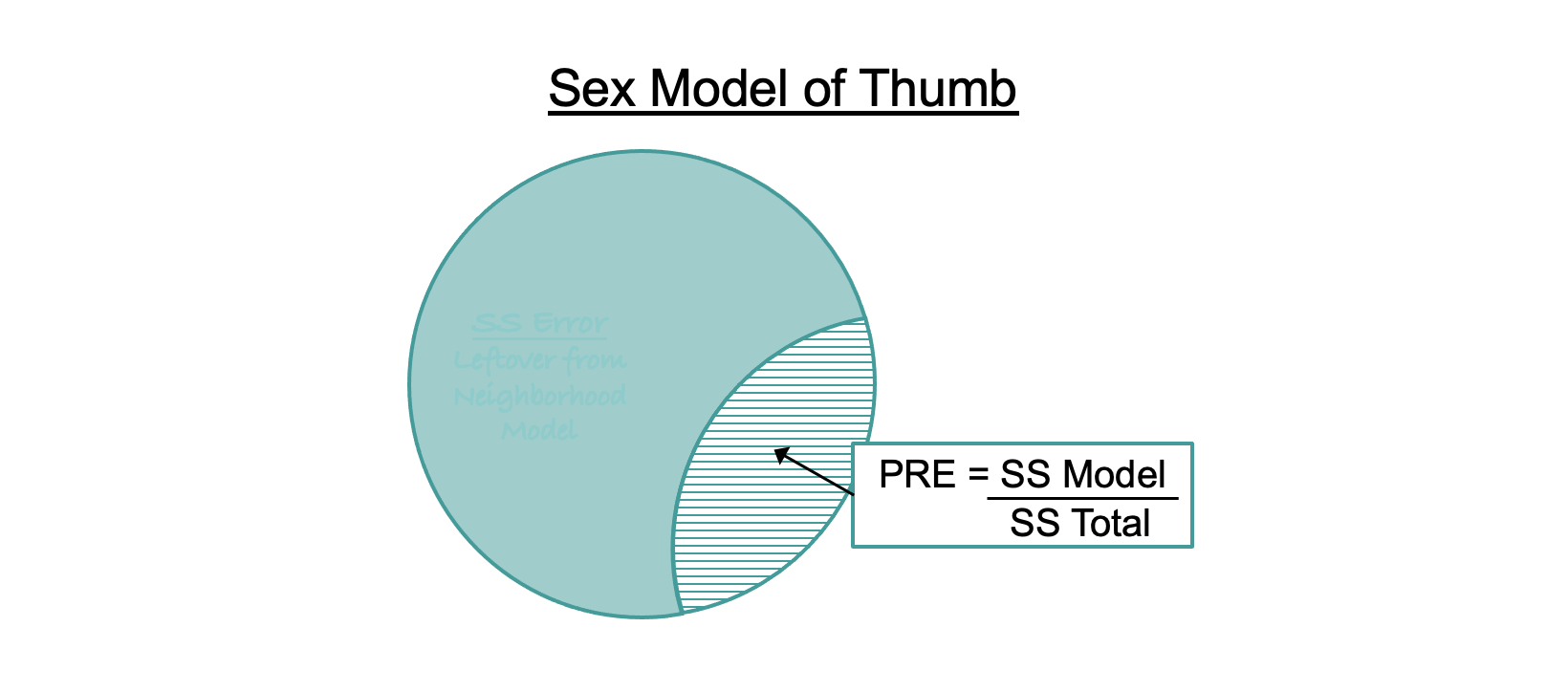
When we calculate PRE this way we are comparing a complex model (e.g., the sex model) to the empty model. Based on this formula, PRE can be interpreted as the proportion of total variation in the outcome variable that is explained by the explanatory variable. It tells us something about the overall strength of our statistical model. For example, in the Fingers data set , the effect of Sex on Thumb accounts for .11 (11%) of the variation in thumb length. Not too shabby.
It is important to remember that SS Model in the numerator of the formula above represents the reduction in error when going from the empty model to the more complex model, which includes an explanatory variable. To make this clearer we can rewrite the above formula like this:
\[\text{PRE}=\frac{(\text{SS}_\text{Total} - \text{SS}_\text{Error})}{\text{SS}_\text{Total}}\]
The numerator of this formula starts with the error from the simple (empty) model (SS Total), and then subtracts the error from the complex model (SS Error) to get the error reduced by the complex model. Dividing this reduction in error by the SS Total yields the proportion of total error in the empty model that has been reduced by the complex model.
The PRE in the ANOVA table above (.11) represents a comparison of the sex model to the empty model, but PRE more generally can represent a comparison of any complex model to one that is simpler. Toward this end, we will add a version of the same formula that is more general:
\[\text{PRE}=\frac{(\text{SS}_\text{Error from Simple Model} - \text{SS}_\text{Error from Complex Model})}{\text{SS}_\text{Error from Simple Model}}\]
Just as a note: PRE goes by other names in other traditions. In the ANOVA tradition (Analysis of Variance) it is referred to as \(\eta^2\), or eta squared. In the next chapter, we will introduce the same concept in the context of regression, where it is called \(R^2\). For now all you need to know is: these are different terms used to refer to the same thing, in case anyone asks you.