9.5 Error from the Height Model
Regardless of model, error from the model (or residuals) are always calculated the same way for each data point:
\[\text{residual}=\text{observed value} - \text{predicted value}\]
For regression models, the predicted value of \(Y_i\) will be right on the regression line. Error, therefore, is calculated based on the vertical gap between a data point’s value on the Y axis (the outcome variable) and its predicted value based on the regression line.
Below we have depicted just 6 data points (in black) and their residuals (firebrick vertical lines) from the Height model.
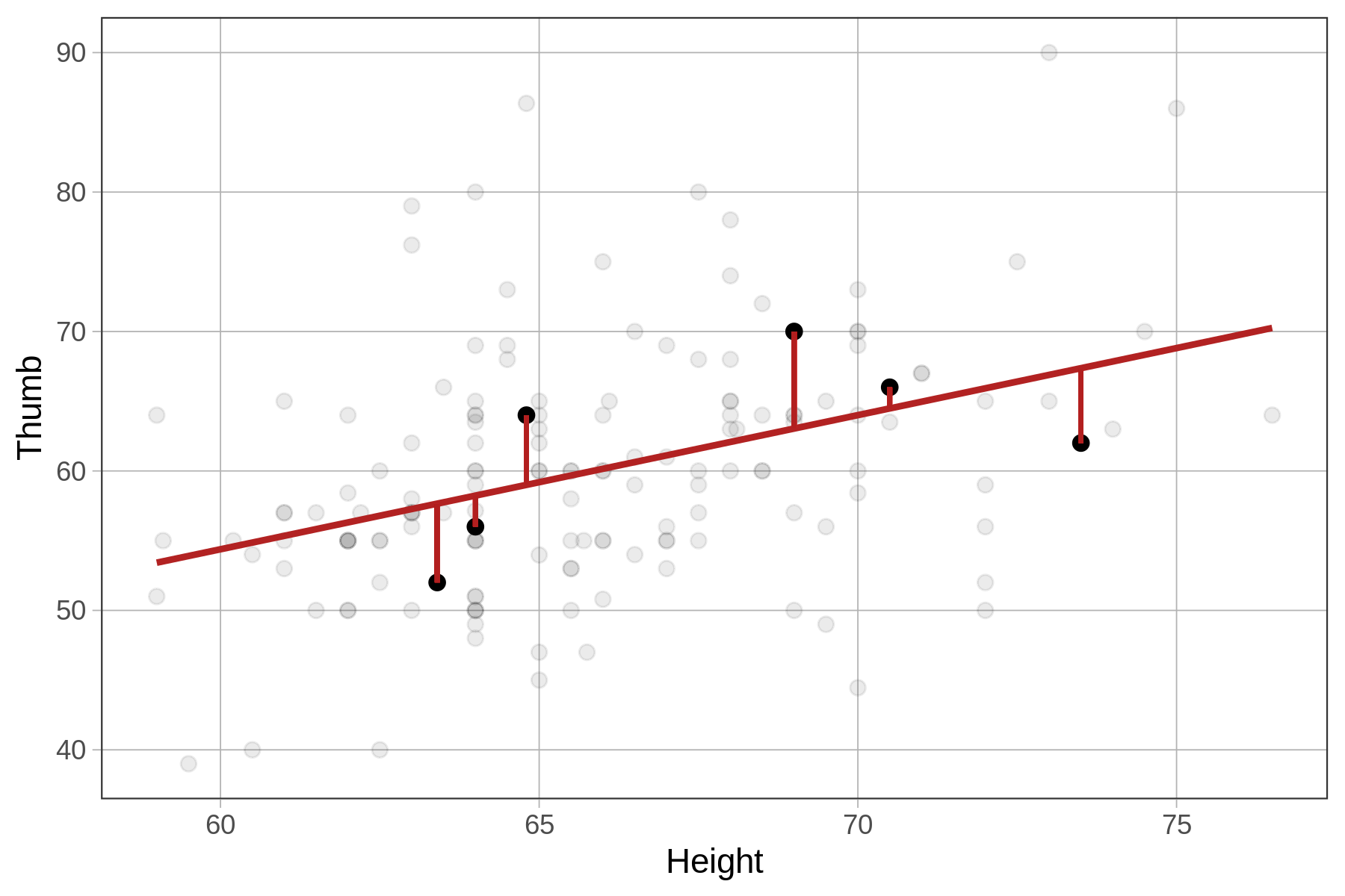
Note that a negative residual (shown below the regression line) means that the data (e.g., Thumb) was lower than the predicted thumb length given the student’s height.
The residuals from the Height model represent the variation in Thumb that is leftover after we take out the part that can be explained by Height. As an example, take a particular student (highlighted in the plot below) with a thumb length of 63 mm. The residual of 7 means that the student’s thumb is 7 mm longer than would have been predicted for this student based on their height.
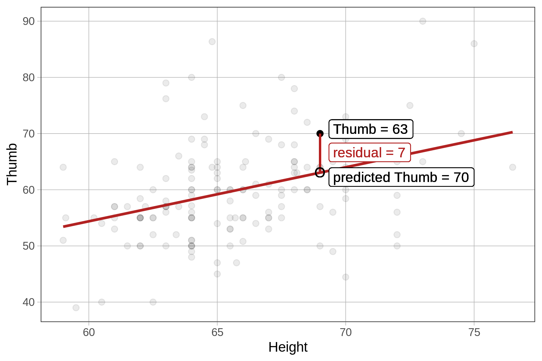
Another way we could say this is: controlling for height, this student’s thumb is 7 mm longer than expected. A positive residual indicates that a thumb is long for a person of that height. A negative residual indicates that a thumb is shorter than expected based on the person’s height. These residuals may prompt us to ask, what other stuff besides Height might account for these differences?
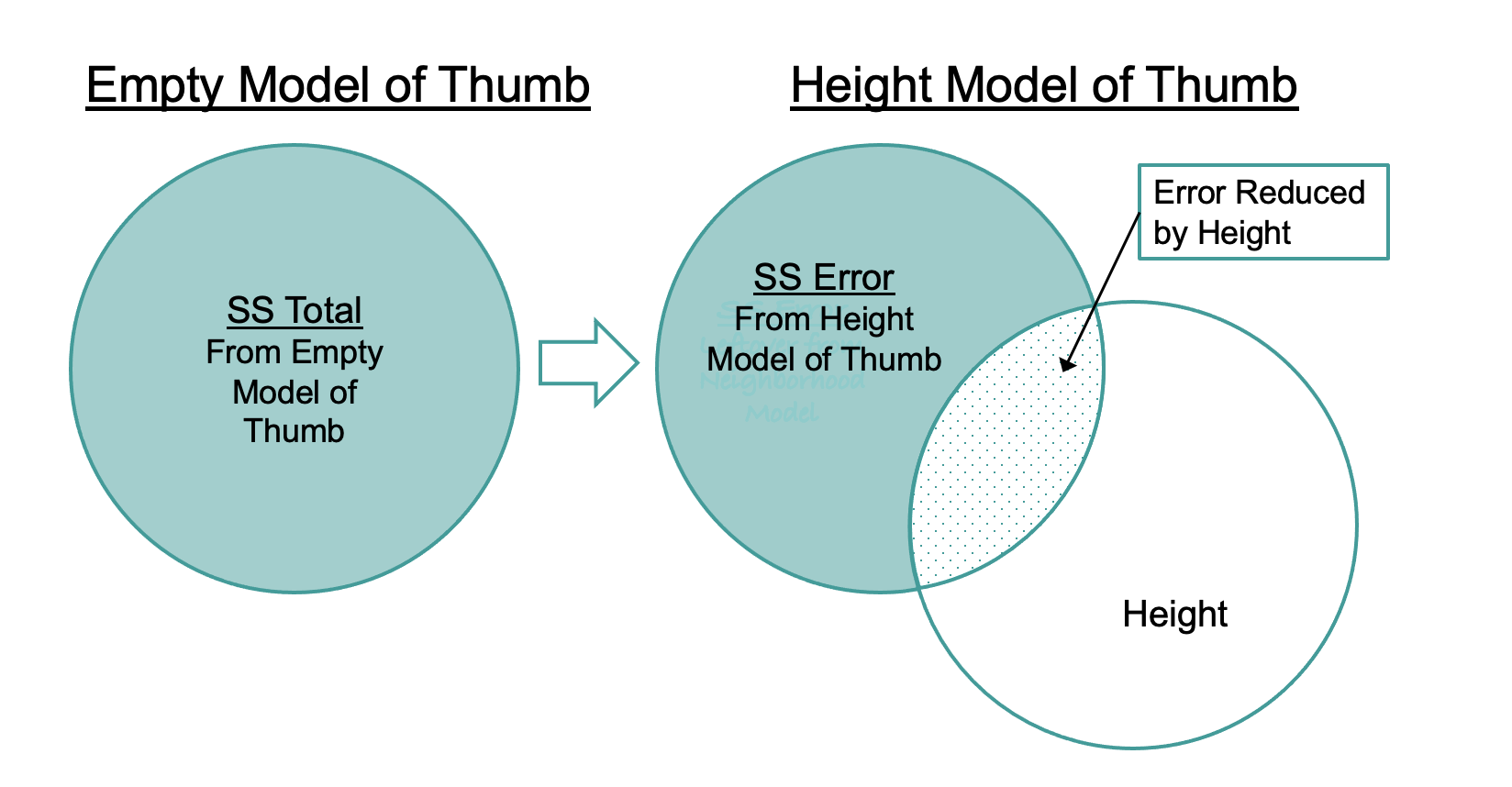
SS Error for the Height Model
Just like for other models we have seen (e.g., the empty model and the group model), the metric we use for quantifying total error from the Height model is the sum of squared residuals from the model, or SS Error. SS Error is calculated from the residuals in the same way as it is for a group model, by squaring and then summing the residuals (see figure below).
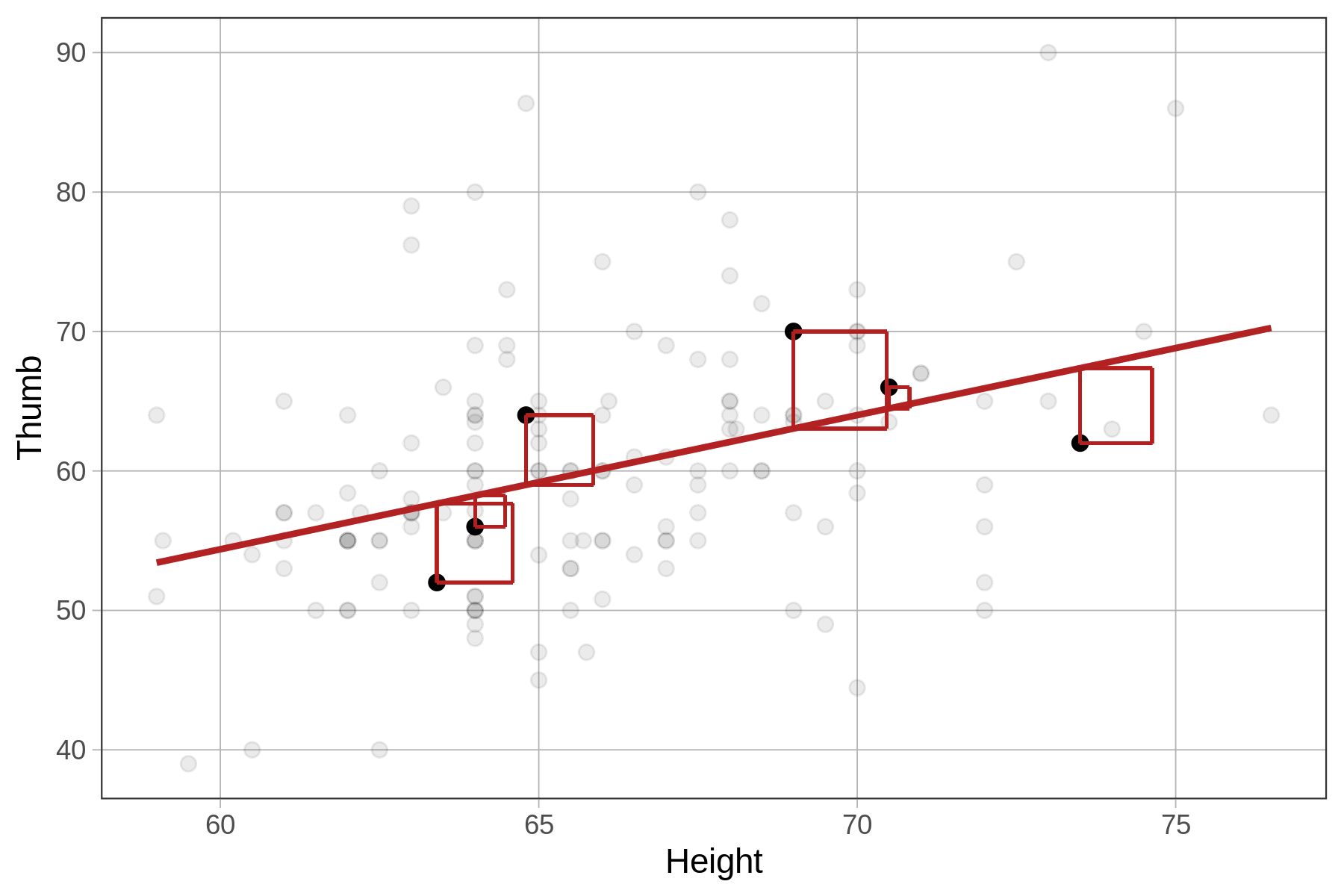
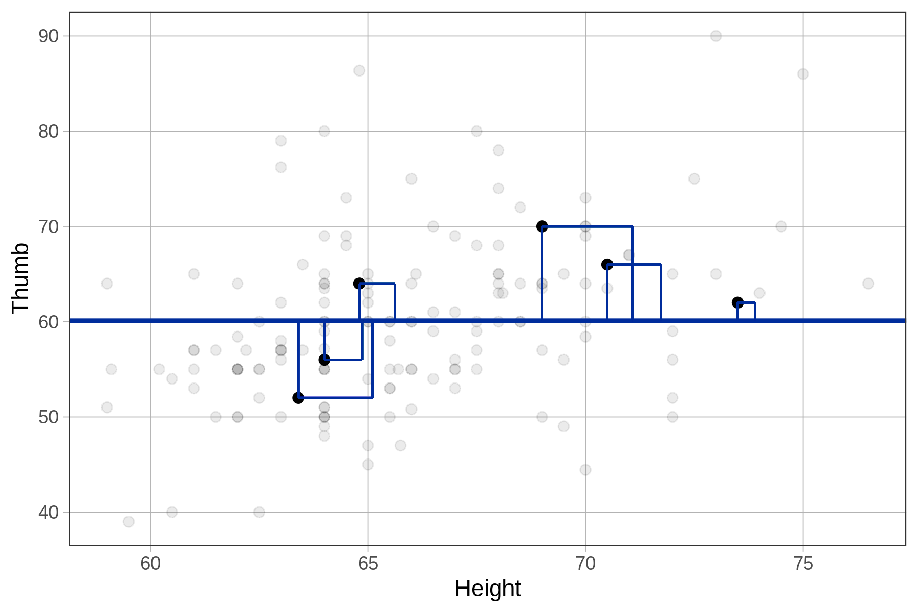
Compare the sums of squares for the empty model (SST) and the height model (SSE) for 6 data points in the figures below.
| SS Total, Sum of Squared Residuals from empty model | SS Error, Sum of Squared Residuals from height model |
|---|---|
|
|
|
Using R to Compare SS for the Height Model and the Empty Model
Just like we did with the group models (e.g., Height2Group model and Sex model), we can use the resid() function to get the residuals from the Height model. We can then square them and sum them to get the SS Error from the model like this:
Height_model <- lm(Thumb ~ Height, data = Fingers)
sum(resid(Height_model)^2)
The code below will calculate SST from the empty model and SSE from the height model. Run it to check our predictions about SSE.
require(coursekata)
# this calculates SST
empty_model <- lm(Thumb ~ NULL, data=Fingers)
print("SST")
sum(resid(empty_model)^2)

# this calculates SSE
Height_model <- lm(Thumb ~ Height, data = Fingers)
print("SSE")
sum(resid(Height_model)^2)
# no test
ex() %>% check_error()[1] "SST"
11880.2109191083
[1] "SSE"
10063.3491457795Notice that the SST is the same as it was for the Height2Group model: 11,880. This is because the empty model hasn’t changed; SST is still based on residuals from the grand mean of Thumb. The SSE (10,063) is smaller than SST because the residuals are smaller (as represented in the figures above by shorter lines). Squaring and summing smaller residuals results in a smaller SSE. The total error has been reduced by this regression model.
Comparing the Regression Line with the Mean
Recall that the mean is the middle of a univariate distribution. It is the balancing point of the distribution, where the residuals are perfectly balanced above and below. In a similar way, the regression line is the middle of a bivariate distribution between two quantitative variables. Just as the sum of the residuals around the mean add up to 0, so too the sum of the residuals around the regression line also add up to 0.
Here’s another cool relationship between the mean and regression line. It turns out that the best-fitting regression line will always pass through a point that is mean of both variables (this is called the point of means). So, if someone’s height is exactly at the mean, their predicted thumb length will also be exactly at the mean.
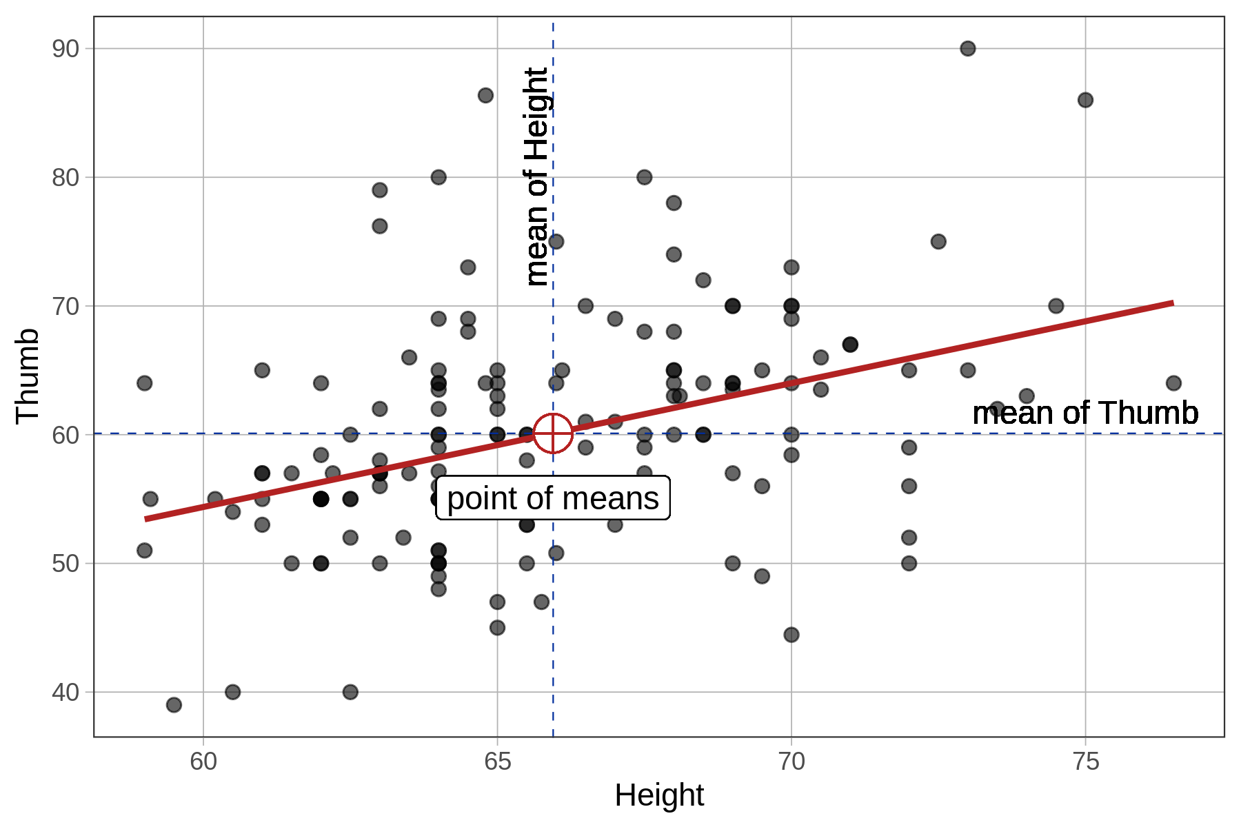
Finally, just as the mean is the point in the univariate distribution at which the SS Error is minimized, the same is true of error around the regression line. The sum of the squared deviations of the observed points is at its lowest possible value around the best-fitting regression line.