8.3 Comparing the Fit of the Two- and Three-Group Models
Examining the Fit of the Three-Group Model
You have already done the following: created the Height3Group categorical explanatory variable; examined the mean thumb lengths of students in each of the three groups; fit the Height3Group model using lm() and interpreted the model parameter estimates; and learned how to represent the three-group model using notation of the GLM.
The final step is to take a look at the ANOVA table so you can compare the fit of the Height3Group model to the empty model. Of course, you know how to do this using supernova(). Go ahead and get the ANOVA table for the Height3Group model.
require(coursekata)

Fingers <- Fingers %>% mutate(
    Height2Group = factor(ntile(Height, 2), 1:2, c("short", "tall")),
    Height3Group = factor(ntile(Height, 3), 1:3, c("short", "medium", "tall"))
)
Height2Group_model <- lm(Thumb ~ Height2Group, data = Fingers)
# creates best fitting Height3Group_model
Height3Group_model <- lm(Thumb ~ Height3Group, data = Fingers)

# use supernova() to print the ANOVA table for this model
Height3Group_model <- lm(Thumb ~ Height3Group, data = Fingers)
supernova(Height3Group_model)
ex() %>% check_output_expr("supernova(Height3Group.model)")Here’s the ANOVA table for the Height3Group model. Just for comparison, we pasted in the table for the Height2Group model right above it.
Height2Group Model
Analysis of Variance Table (Type III SS)
Model: Thumb ~ Height2Group

                               SS  df      MS      F    PRE     p
----- --------------- | --------- --- ------- ------ ------ -----
Model (error reduced) |   830.880   1 830.880 11.656 0.0699 .0008
Error (from model)    | 11049.331 155  71.286
----- --------------- | --------- --- ------- ------ ------ -----
Total (empty model)   | 11880.211 156  76.155
Height3Group Model
Analysis of Variance Table (Type III SS)
Model: Thumb ~ Height3Group

                               SS  df      MS      F    PRE     p
----- --------------- | --------- --- ------- ------ ------ -----
Model (error reduced) |  1690.440   2 845.220 12.774 0.1423 .0000
Error (from model)    | 10189.770 154  66.167
----- --------------- | --------- --- ------- ------ ------ -----
Total (empty model)   | 11880.211 156  76.155
Later on or in more advanced classes you will learn how to compare these two models directly. But for now, we will only compare each model to the empty model.
Improving Models by Adding Parameters
You probably noticed in the previous section that the three-parameter Height3Group model explained more variation than the Height2Group model; that is, it reduced the unexplained error more than the Height2Group model when compared with the empty model. You can see that by comparing the PREs (.14 versus .07, respectively).
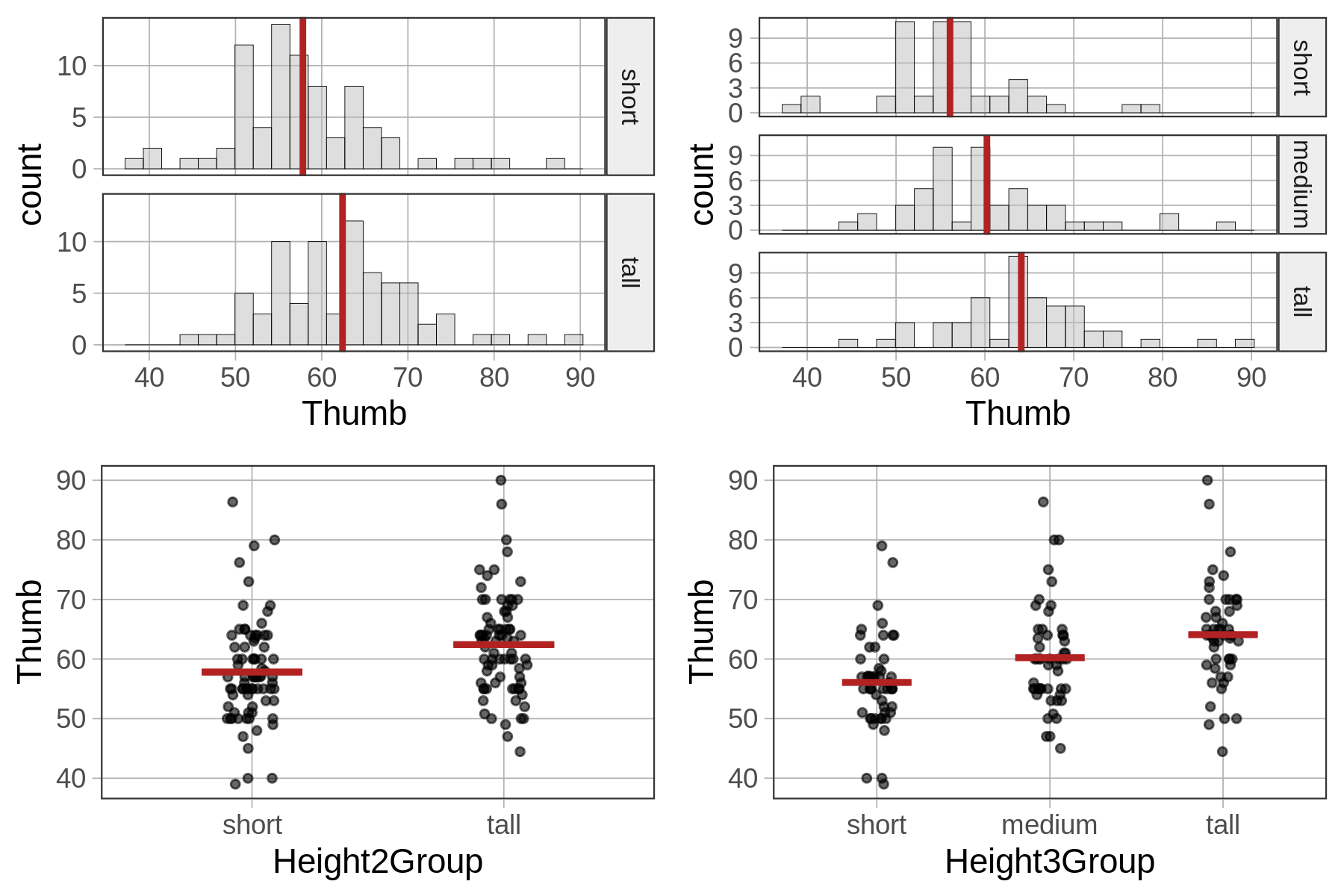
If we look at histograms and jitter plots for the two-group model and the three-group model (below) you can get a sense of why this is. By adding more categories for height we are able to reduce the error variation around the mean height for each group.
In general, the more parameters we add to a model the less leftover error there is after subtracting out the model. This isn’t always the case, but typically more complex models do have higher PREs. Because the goal of the statistician is to reduce error, more complexity might seem like a good thing. And it is, but only to a point.
Let’s do a little thought experiment. You know already that the three-group model explained more variation than the two-group model. The four-group model would explain more than the three-group. And so on. What would happen if we kept splitting into more groups until each person was in their own group?
If each person were in their own group, the error would be reduced to 0. Why? Because each person would have their own parameter in the model. If each person had their own parameter, then the predicted score for that person would just be the person’s actual score. And there would be no residual between the predicted and actual score. All the variation would be explained by the model!
There are two problems with this. First, even though the model fits our data perfectly, it would not fit if we were to choose another sample (because the people would be different). Second, the purpose of creating a more complex model is to help us understand the Data Generating Process. It’s okay to add a little complexity to a model if it leads to better understanding. But if we have as many parameters as we have people, we have added a lot of complexity without contributing to our understanding of the DGP.
Although we can improve model fit by adding parameters to a model, there is always a trade-off involved between reducing error (by adding more parameters to a model), on one hand, and increasing the intelligibility, simplicity, and elegance of a model, on the other.
This is a limitation of PRE as a measure of our success. If we get a PRE of .40, for example, that would be quite an accomplishment if we had only added a single parameter to the model. But if we had achieved that level by adding 10 parameters to the model, well, it’s just not as impressive. Statisticians sometimes call this “overfitting.”
There is a quote attributed to Einstein that sums up things pretty well: “Everything should be made as simple as possible, but not simpler.” A certain amount of complexity is required in our models just because of complexity in the world. But if we can simplify our model so as to help us make sense of complexity, and make predictions that are “good enough,” that is a good thing.