4.6 Things that Affect P-Value

What If The Sample $b_1$ were 10?

The sample $b_1$ in the tipping experiment was $6.05. Based on the sampling distribution we created of $b_1$ assuming the empty model, we calculated the probability of getting a sample with a $b_1$ as extreme or more extreme than $6.05 as approximately .08. Based on our alpha criterion of .05, we decided that $6.05 was not unlikely to have resulted from the empty model, and so we did not reject the empty model.

Imagine, now, that the mean difference between the smiley and control groups was $10. How would that affect the p-value, and how would it affect our decision about whether or not to reject the empty model of the DGP?

P-value is definitely affected by how far the observed $b_1$ is from 0. Since $10 is further away from 0 than $6.05 is from 0, when $b_1=10$, we get a smaller p-value. The further away the $b_1$ is from 0, the lower the p-value, meaning the less likely the observed $b_1$ is to have been produced by the empty model.

Standard Error and P-value

The distance between $b_1$ and 0 (or the hypothesized ${\beta }_1$) is not the only thing that affects p-value. The other important factor is the width of the sampling distribution, which can be quantified using standard error.

The standard error is the standard deviation of a sampling distribution.

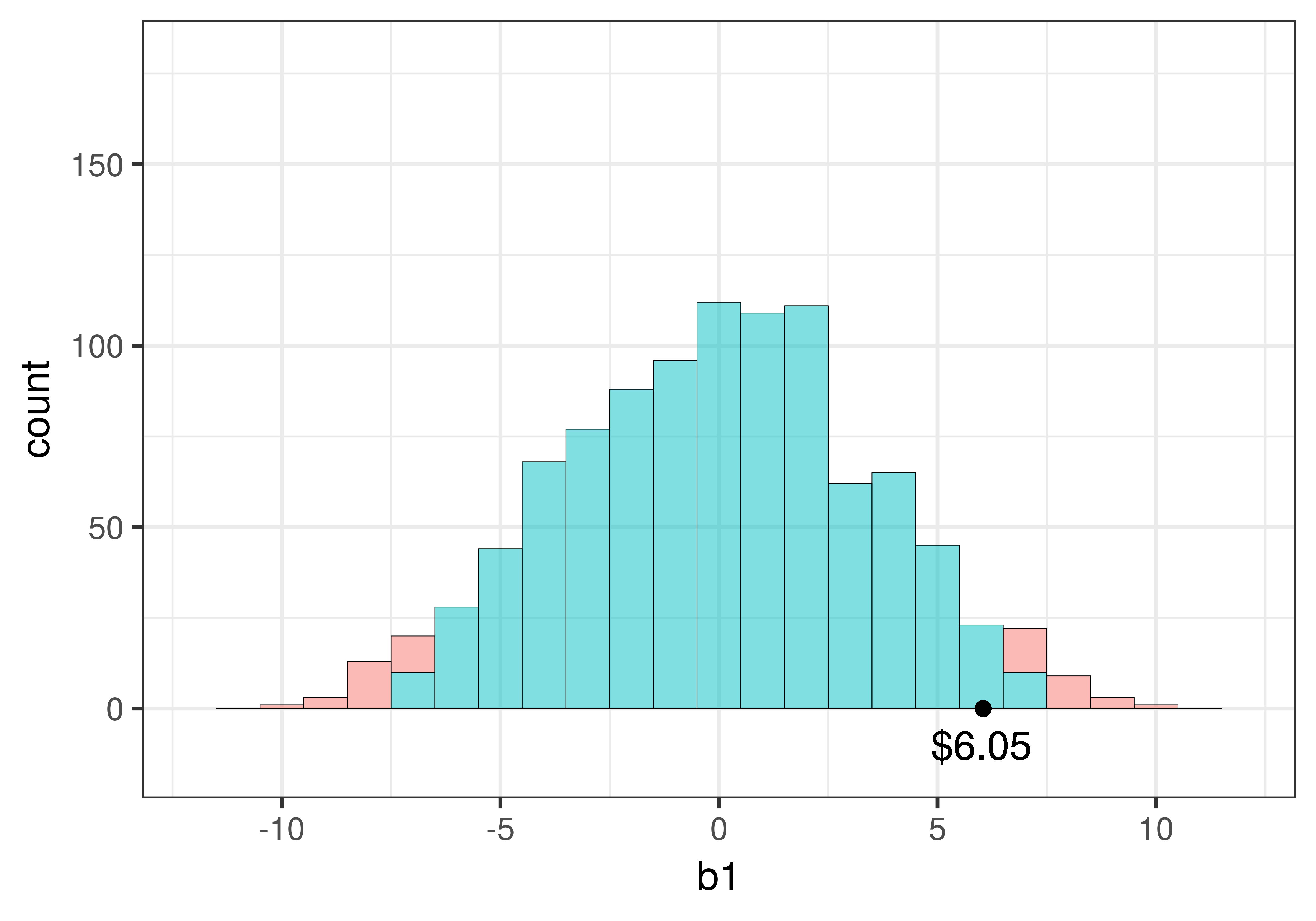
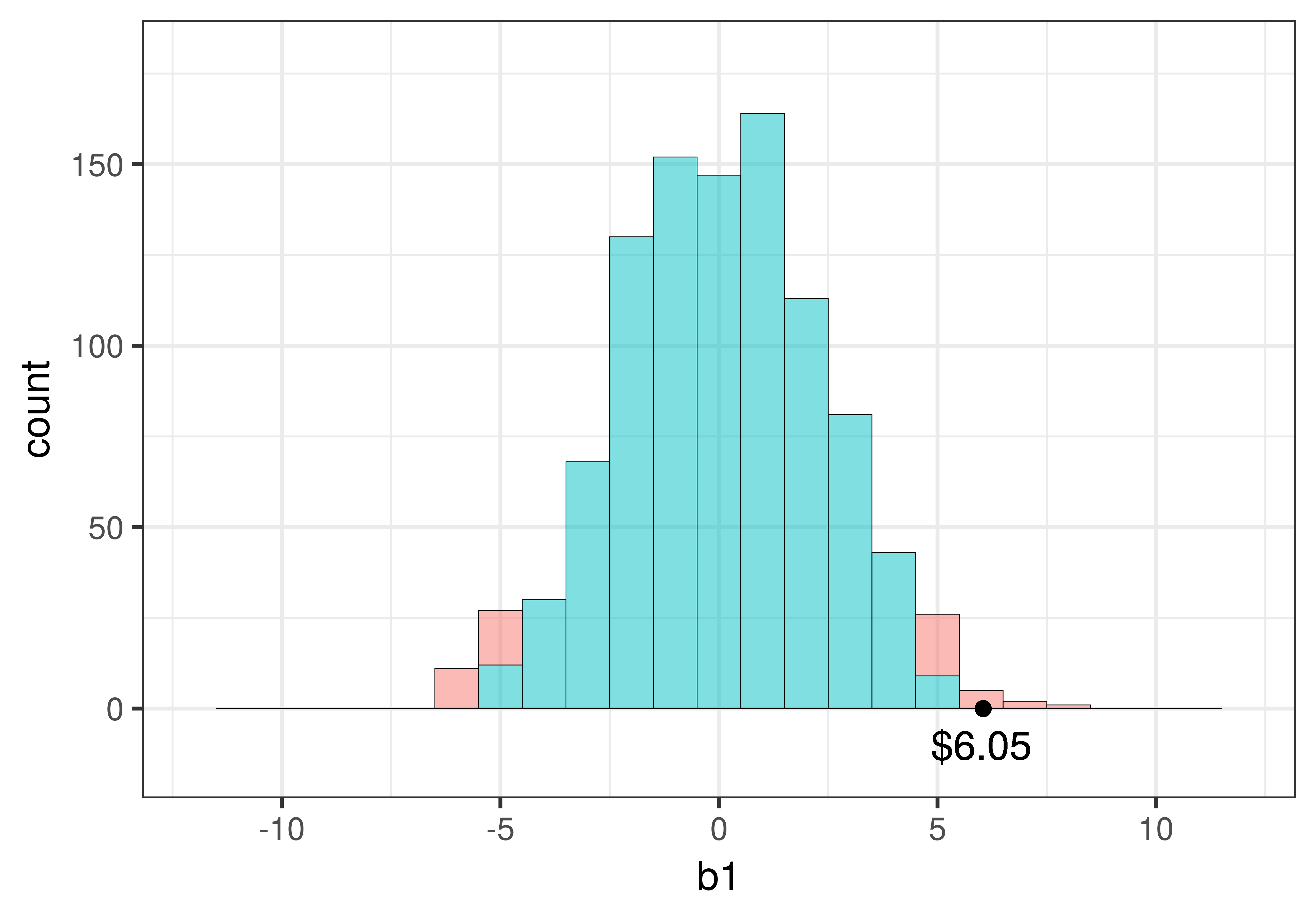
Take a look at the two simulated sampling distributions in the figure below. The one on the left is the one we created using shuffle() for the tipping experiment. The one on the right is similar in every way but the spread is considerably narrower. Both have a roughly normal shape, both consist of 1000 $b_1$s, and both distributions are centered at 0. But the standard error is smaller for the distribution on the right.

The standard error can make a big difference in our evaluation of the empty model. If it is smaller, we will have an easier time rejecting the empty model, because whatever estimate we get for $b_1$, it will be more likely to be in the upper or lower .025 of the sampling distribution.

Sample Size and Standard Error

We have demonstrated how p-value is affected by standard error (the width of the sampling distribution). But so what? Do we really have any control of the width of the sampling distribution? Actually, we do, if we are the ones designing the study and collecting the data.

There are two main things that affect standard error: (1) the standard deviation of the DGP and (2) the size of your sample. As a researcher, you have no control over how variable the DGP is, but because you can decide to collect more or less data, you do have control over the size of your sample.

Let’s explore how sample size might impact the sampling distribution of $b_1$. Consider an alternate universe where the researchers who did the tipping study collected data from 88 tables instead of just 44. Imagine that the sample of $n=88$ had the same group difference ($b_1=6.05$) and the same standard deviation for Tip as the original study but just happened to have more tables in the sample.

To simulate this imaginary situation, we made a new data frame called TipExp2 that simply has two copies of each table in the original TipExperiment). We can run str() on this new data frame to see what it looks like.

str(TipExp2)

'data.frame':   88 obs. of  3 variables:
 $ ServerID : int  1 2 3 4 5 6 7 8 9 10 ...
 $ Tip      : atomic  39 36 34 34 33 31 31 30 30 28 ...
  ..- attr(*, "format.spss")= chr "F8.0"
 $ Condition: Factor w/ 2 levels "Control","Smiley Face": 1 1 1 1 1 1 1 1 1 1 ...

Use the code window below to compare the new data frame (TipExp2) to the original one (TipExperiment). In particular, look at the overall mean and standard deviation of the outcome variable Tip, for each data set, and also fit the Condition model to see what the best-fitting $b_1$ is for the two data sets.

You can check your results against the table below. These numbers match up very closely across the two samples for a reason: both data frames include the same 44 tables, either one time or two.

Sample Size	Mean Tip	SD Tip	$b_1$
n=44	30.0	11.3	6.05
n=88	30.0	11.3	6.05

Although sample size doesn’t necessarily affect the mean, standard deviation, or $b_1$ – these are all features of the sample distribution – it will affect the width of the sampling distribution. Let’s explore this idea by creating two sampling distributions, one for the n=44 sample, the other for n=88. We will use the shuffle() function again to simulate the empty model, where ${\beta }_1=0$.

Here is code to create the two sampling distributions of $b_1$, one for the data set with 44 tables, the other with 88 tables.

sdob44 <- do(1000) * b1(shuffle(Tip) ~ Condition, data = TipExperiment)
sdob88 <- do(1000) * b1(shuffle(Tip) ~ Condition, data = TipExp2)

We then ran this code to produce histograms of the two sampling distributions of $b_1$.

gf_histogram(~ b1, data = sdob44, fill = ~middle(b1,.95), binwidth=.3, show.legend = FALSE) %>%
gf_lims(x = c(-12, 12), y = c(0,70))
 
gf_histogram(~ b1, data = sdob88, fill = ~middle(b1,.95), binwidth=.3, show.legend = FALSE) %>%
gf_lims(x = c(-12, 12), y = c(0,70))

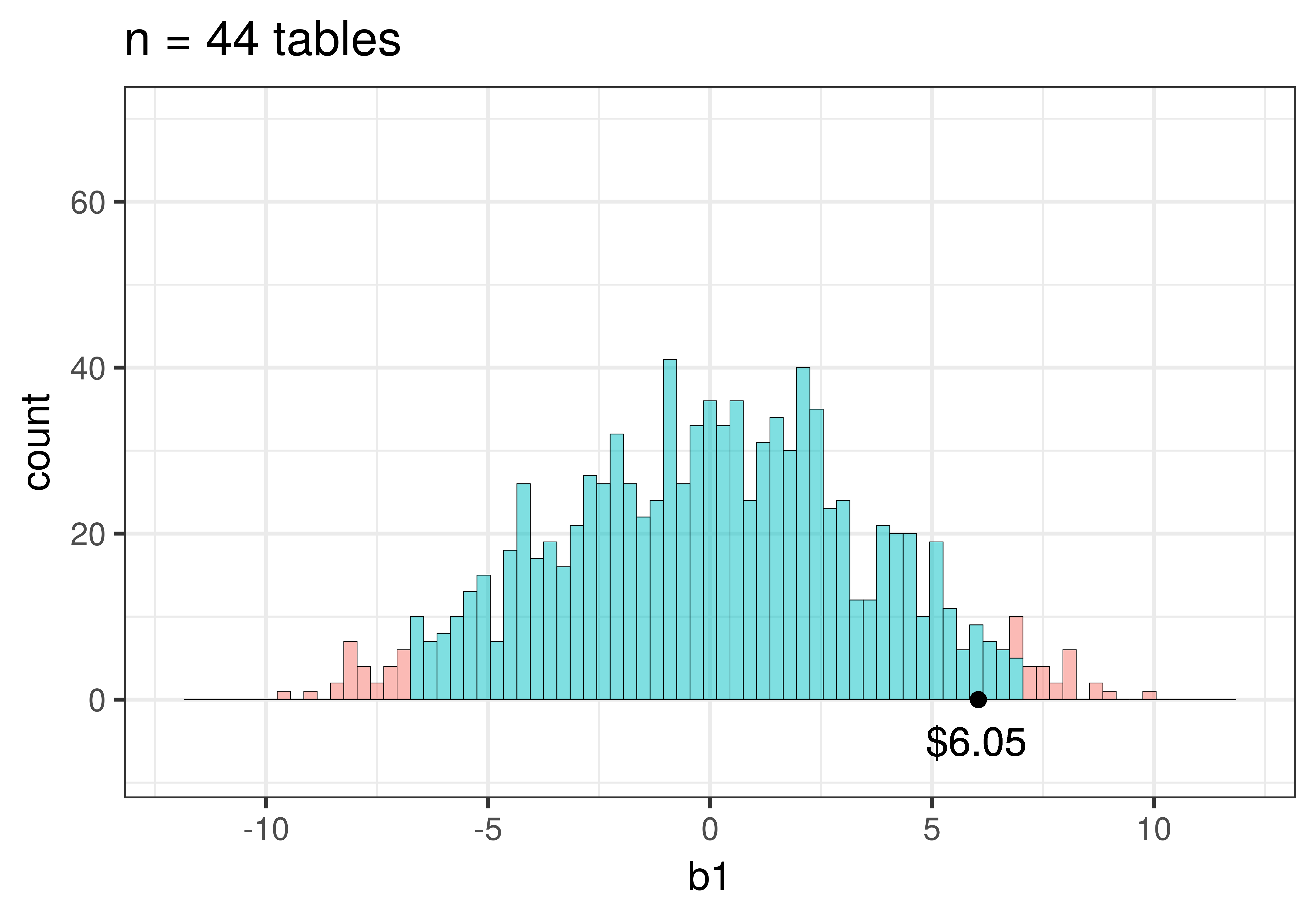
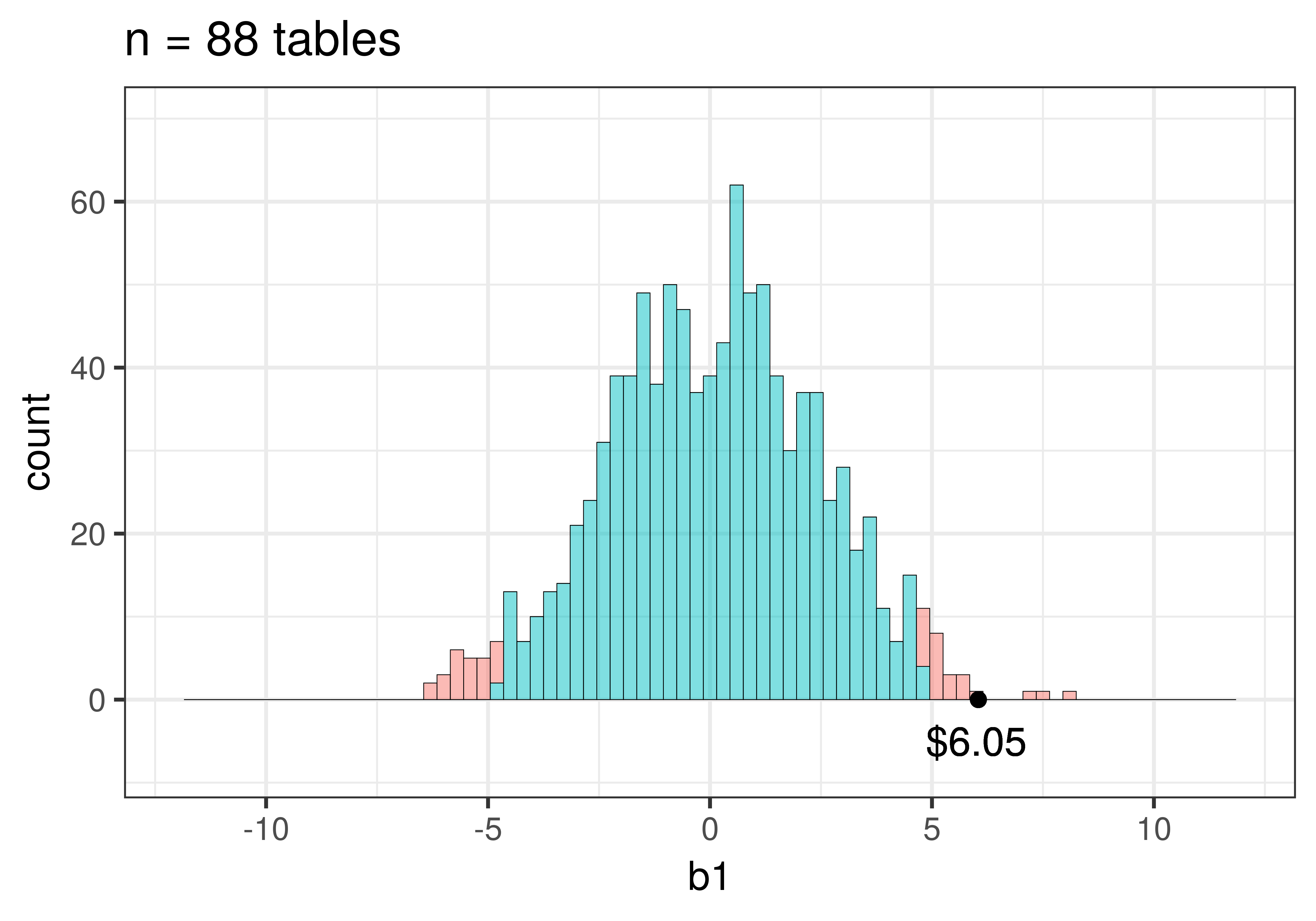
Note that we added this code (gf_lims(x = c(-12, 12), y = c(0,70))) to make sure the scales are the same for the two histograms so you could more easily compare them. You may recognize these histograms – they are the same ones we presented above, but now you know how we made them.

Notice how the sampling distribution varies much less when based on samples of 88 tables than it does for 44 tables. Use the code window below to calculate the standard errors for the two sampling distributions. (Hint: The standard error is the standard deviation of a sampling distribution.)

[1] 3.534982
[1] 2.413229

Even though both sampling distributions are roughly normal and centered at 0 (after all, the empty model has a ${\beta }_1=0$), the standard error is smaller in the sampling distribution of $b_1$s based on samples of 88 tables (around 2.4 versus 3.5).

It turns out that larger sample sizes always produce smaller standard errors (narrower sampling distributions), because in larger samples, it is much harder to get an extreme $b_1$ by chance alone. To get an extreme $b_1$ by chance alone you would need a lot of the big tipping tables to get randomly assigned to one condition and the small tipping tables to the other. If you only had two tables, this is quite easy to do! If you had just 4 tables, this is also not too hard to do. But as you increase the number of tables, it’s hard to keep that pattern up. It’s the same reason why it’s easy to flip 2 heads in a row but very hard to flip 44 heads in a row. It’s easy to randomly assign a few big tippers to one condition but hard to randomly assign 40 big tippers to one condition.

Standard Error and Rejecting the Empty Model

Even though the sample $b_1$ is the same in both situations, when the standard error is smaller, that makes our sample seem less likely to have been generated by the empty model. In general, the p-value for a sample statistic will be smaller as the sample size gets larger.

Let’s take a look at the p-value, which can be found in the ANOVA table.

Analysis of Variance Table (Type III SS)
Model: Tip ~ Condition (From TipExperiment)

                              SS df      MS     F    PRE     p
----- ----------------- -------- -- ------- ----- ------ -----
Model (error reduced) |  402.023  1 402.023 3.305 0.0729 .0762
Error (from model)    | 5108.955 42 121.642                   
----- ----------------- -------- -- ------- ----- ------ -----
Total (empty model)   | 5510.977 43 128.162                   

Analysis of Variance Table (Type III SS)
Model: Tip ~ Condition (From TipExp2)

                               SS df      MS     F    PRE     p
----- ----------------- --------- -- ------- ----- ------ -----
Model (error reduced) |   804.045  1 804.045 6.767 0.0729 .0109
Error (from model)    | 10217.909 86 118.813                   
----- ----------------- --------- -- ------- ----- ------ -----
Total (empty model)   | 11021.955 87 126.689                   

Notice that the p-value from the original data is .08 but the p-value from twice as much data is .01. Below we have depicted the p-value (in purple) by coloring the tails beyond the sample $b_1$ in each of these sampling distributions.