3.11 Conceptualizing SS Model
There is another, more direct, way to calculate SSM that can help you better understand the concept of SSM.
The empty model makes a prediction for each home in Ames (depicted as the blue horizontal line below). The complex model also makes a prediction for each home (depicted as firebrick horizontal lines). The differences between these two predictions, for each neighborhood, are depicted in the jitter plot below.
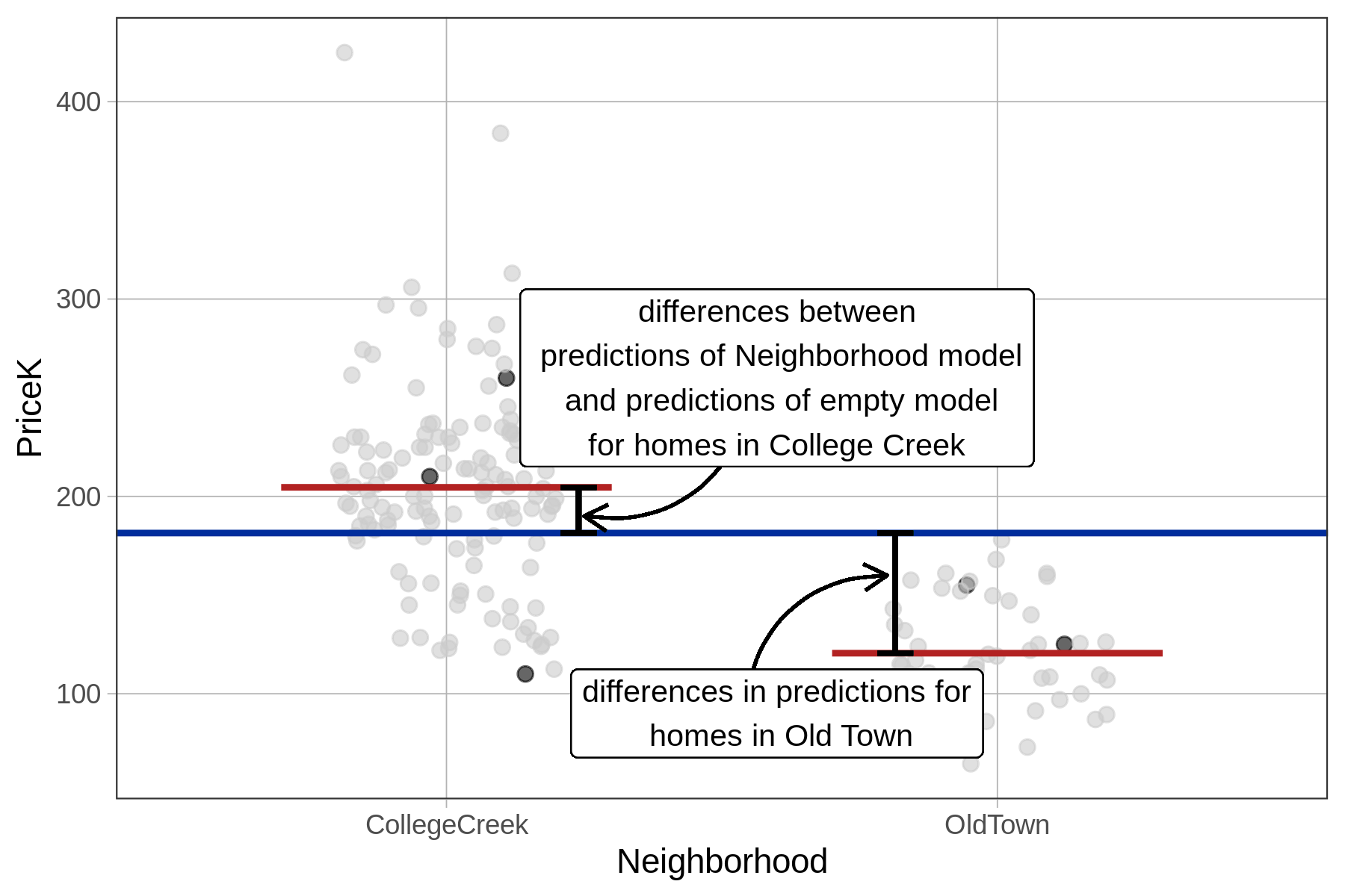
On average, error is reduced as we move from using the predictions of the empty model to using the predictions of the complex model. Below we have zoomed in on a College Creek home (that sold for $260K) to show you a case where the neighborhood model’s prediction is closer to the actual sale price than the empty model’s prediction. The “reduction in error” is based on how much the empty model’s residual has been reduced.
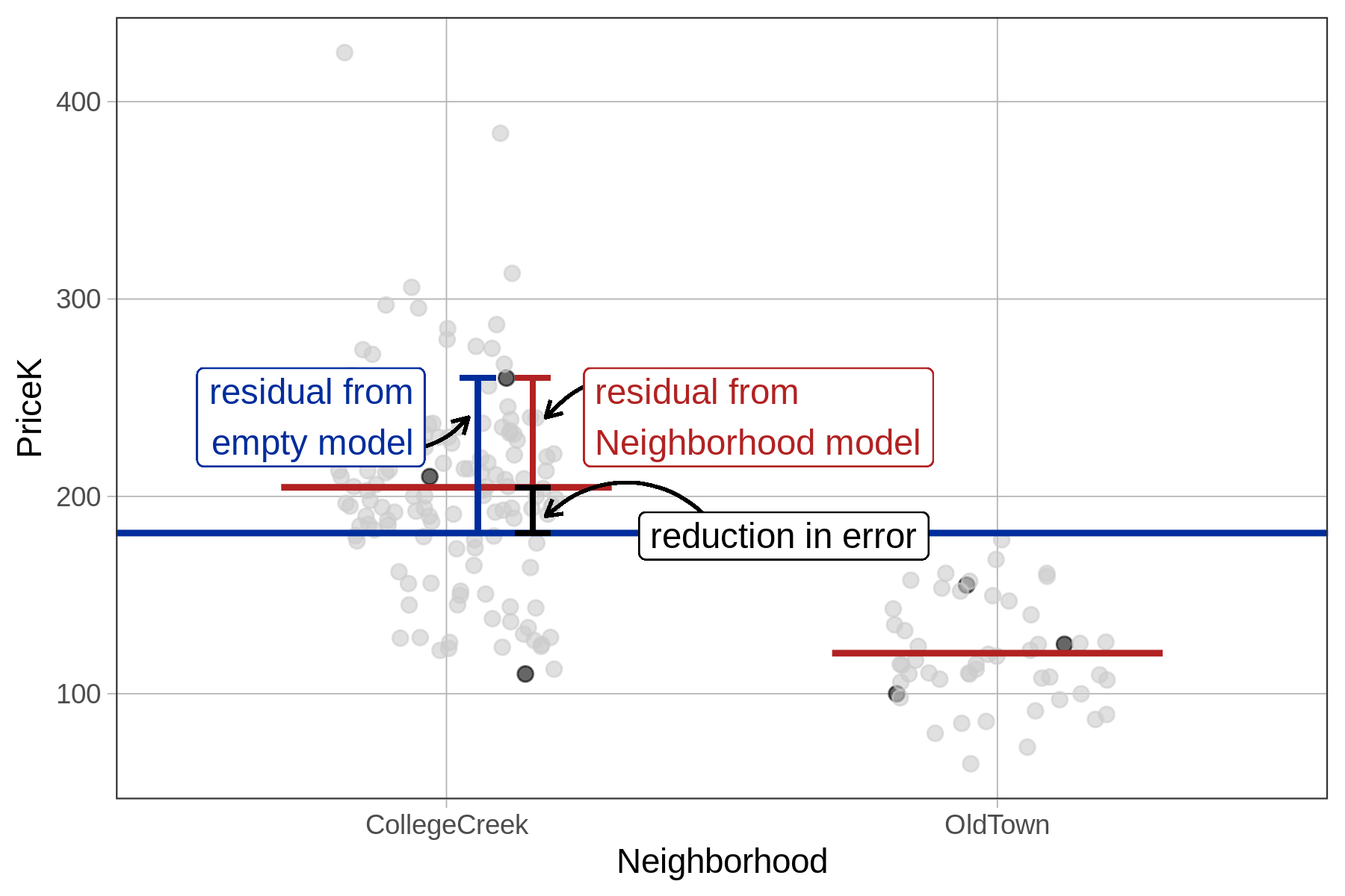
The amount by which the total error is reduced by the neighborhood model over the empty model (SSM) is the difference between the two model predictions, squared and summed across all data points.
In the code window below, try calculating the SS Model for the neighborhood model.
require(coursekata)
empty_model <- lm(PriceK ~ NULL, data=Ames)
Neighborhood_model <- lm(PriceK ~ Neighborhood, data = Ames)
# This generates predictions from empty model
Ames$empty_predict <- predict(empty_model)

# This generates predictions from Neighborhood model
Ames$Neighborhood_predict <- predict(Neighborhood_model)

# Here are the differences
# Square and sum these differences to calculate SSM
(Ames$empty_predict - Ames$Neighborhood_predict)
# This generates predictions from empty model
Ames$empty_predict <- predict(empty_model)

# This generates predictions from Neighborhood model
Ames$Neighborhood_predict <- predict(Neighborhood_model)

# Here are the differences
# Square and sum these differences to calculate SSM
sum((Ames$empty_predict - Ames$Neighborhood_predict)^2)
ex() %>% check_function('sum') %>%
check_result() %>% check_equal()260904.011627901This value matches the SS Model as seen in the ANOVA table we have re-printed below.
Analysis of Variance Table (Type III SS)
 Model: PriceK ~ Neighborhood

                                 SS  df         MS       F    PRE     p
 ----- --------------- | ---------- --- ---------- ------- ------ -----
 Model (error reduced) | 260904.012   1 260904.012 128.068 0.4117 .0000
 Error (from model)    | 372813.204 183   2037.231
 ----- --------------- | ---------- --- ---------- ------- ------ -----
 Total (empty model)   | 633717.215 184   3444.115
Comparing Models with Sums of Squares
Let’s now compare the ANOVA tables between the neighborhood model and the home size model.
The code below generates the ANOVA table for the neighborhood model. Write some additional code to generate the ANOVA table for the home size model.
require(coursekata)
# Produces ANOVA table for Neighborhood model
Neighborhood_model <- lm(PriceK ~ Neighborhood, data = Ames)
supernova(Neighborhood_model)

# Write additional code to produce ANOVA table for HomeSizeK model
HomeSizeK_model <- lm(PriceK ~ HomeSizeK, data = Ames)
# Produces ANOVA table for Neighborhood model
Neighborhood_model <- lm(PriceK ~ Neighborhood, data = Ames)
supernova(Neighborhood_model)

# Write additional code to produce ANOVA table for HomeSizeK model
HomeSizeK_model <- lm(PriceK ~ HomeSizeK, data = Ames)
supernova(HomeSizeK_model)
ex() %>% check_function("supernova", 2) %>%
  check_result() %>% check_equal()
Analysis of Variance Table (Type III SS)
Model: PriceK ~ Neighborhood

                                 SS  df         MS       F    PRE     p
 ----- --------------- | ---------- --- ---------- ------- ------ -----
 Model (error reduced) | 260904.012   1 260904.012 128.068 0.4117 .0000
 Error (from model)    | 372813.204 183   2037.231
 ----- --------------- | ---------- --- ---------- ------- ------ -----
 Total (empty model)   | 633717.215 184   3444.115
Analysis of Variance Table (Type III SS)
 Model: PriceK ~ HomeSizeK

                                 SS  df         MS       F    PRE     p
 ----- --------------- | ---------- --- ---------- ------- ------ -----
 Model (error reduced) | 374764.505   1 374764.505 264.843 0.5914 .0000
 Error (from model)    | 258952.711 183   1415.042
 ----- --------------- | ---------- --- ---------- ------- ------ -----
 Total (empty model)   | 633717.215 184   3444.115
Both models have the same SST because they use the same outcome variable (PriceK). The better model is the home size model because it reduces error in the outcome variable more than the neighborhood model. We can see this because it has a lower SSE and a higher SSM. And of course, SSE and SSM are perfectly related: as one goes up, the other must go down, because they always add up to SST.
The HomeSizeK model reduces error by 374,765 squared dollars. Huh? What’s a squared dollar? Is that a lot of squared dollars or just a small amount? Squared dollars are hard to interpret. In fact, squares of most units are hard to interpret. This is why we usually use two other statistics when comparing models: PRE and F.