3.4 Error from the Neighborhood Model
In the previous chapter, we calculated residuals from the empty model of PriceK by starting with the actual sales price of each home, and then subtracting the predicted value based on the model. In the empty model, all homes had the same predicted value.
For the Neighborhood model of PriceK we will use the same method, the only difference being that this time there will be two different predictions from the model depending on which neighborhood the home is in. Still, the predicted sales price of each home, which depends on neighborhood, is subtracted from the actual sales price to get the residuals.
The residuals for 6 example homes are represented in the plots below for both the empty model (left) and Neighborhood model (right). Notice that the placement of the 6 data points is the same from one model to the other; the actual prices of these homes don’t change.
| Residuals from the Empty Model | Residuals from the Neighborhood Model |
|---|---|
|
|
|

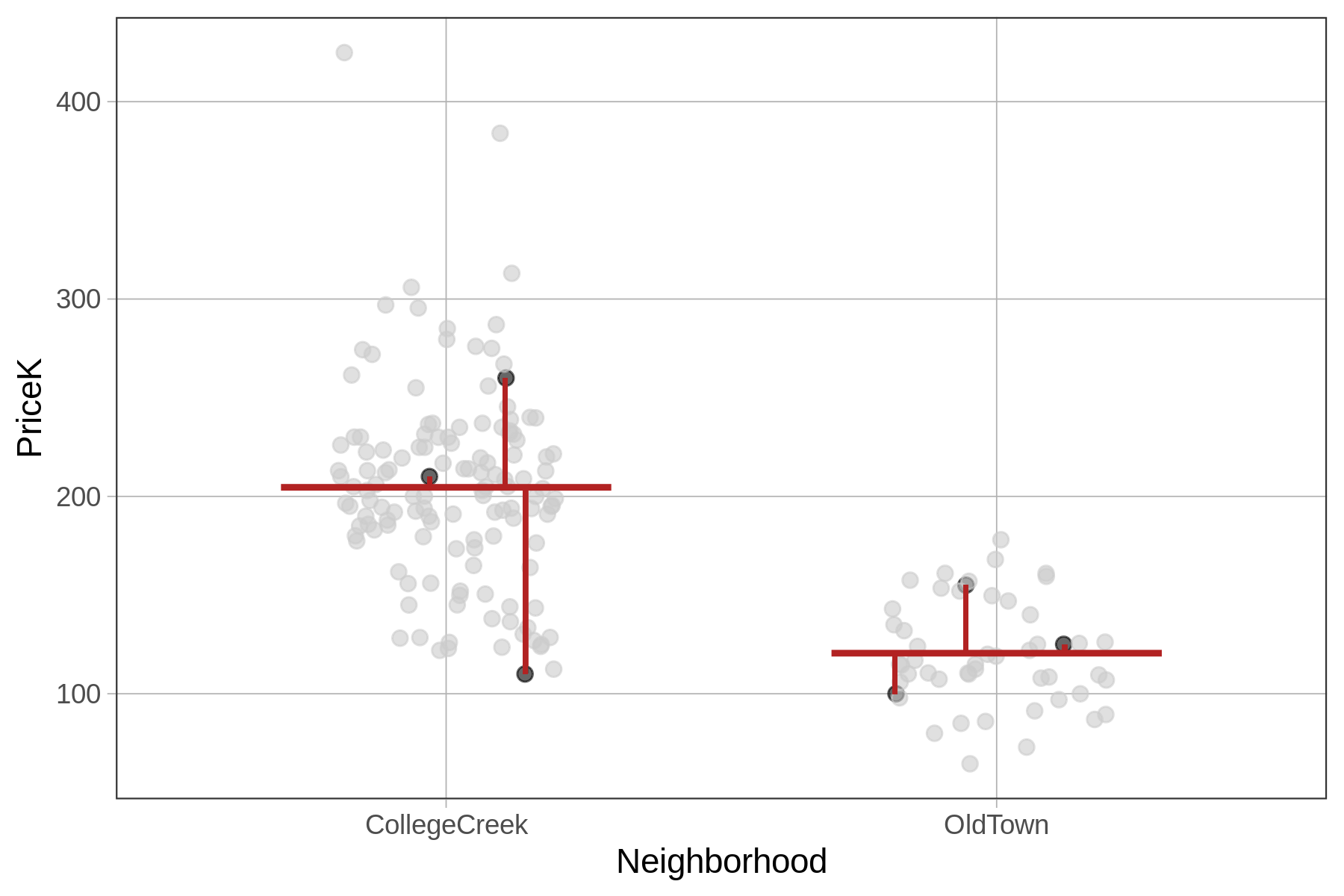
The predictions and residuals of the two models, however, are different. For the empty model, each home’s residual is calculated in relation to the mean PriceK of all homes in the data set. For the Neighborhood model, each home’s residual is calculated in relation to the predicted PriceK for its neighborhood.
Something to keep in mind as well is that looking at residuals can help you interpret your data. Take, for example, the home in Old Town, circled in the plots below. Looking at residuals can help you see something interesting about this home.
| In relation to the empty model, this home sold for a below–average price. |
In relation to the Neighborhood model, the same home sold for a slightly above–average price given the neighborhood it is in.
|
|---|---|
|
|
|


Using R to Calculate Residuals from the Neighborhood Model
Just as we earlier used the predict() function to assign a predicted PriceK to each home in the data frame, we can use the resid() function to calculate the residual for each home. We’ve done that with the code below, and printed out the data table for just the 6 houses we have been looking at.
Ames$Neighborhood_predict <- predict(Neighborhood_model)
Ames$Neighborhood_resid <- resid(Neighborhood_model)
head(select(Ames, Neighborhood, PriceK, Neighborhood_predict, Neighborhood_resid))
Neighborhood PriceK Neighborhood_predict Neighborhood_resid
1 CollegeCreek 260 204.5960 55.403985
2 CollegeCreek 210 204.5960 5.403985
3 OldTown 155 120.5555 34.444510
4 OldTown 125 120.5555 4.444510
5 CollegeCreek 110 204.5960 -94.596015
6 OldTown 100 120.5555 -20.555490