Chapter 7 - Introduction to Multivariate Models

7.1 Models with Two Explanatory Variables

Up to now we have limited ourselves to models with just one explanatory or predictor variable (we will call these single-predictor models). For example, in prior chapters we have modeled home prices in the Ames data frame as a function of neighborhood (Price = Neighborhood + Other Stuff) and as a function of square footage in the house (Price = Home Size + Other Stuff).

Most of the outcomes we are interested in, however, are the result of multiple variables. Putting aside for now the question of whether one variable causes variation in another, it certainly is the case that in data, most outcomes can be explained by more than one variable, and it is usually the case that the more explanatory variables you add to a model, the greater proportion of variation in the outcome variable will be explained.

In this chapter we will focus on specifying, fitting, and interpreting multivariate models. As before, we will be working with the General Linear Model, just extending it to include more than one predictor variable. As you will see, you will mostly be able to apply what you’ve learned before to help you understand these new models.

It is still going to be the case, for example, that DATA = MODEL + ERROR. But as we add more variables to the MODEL, we will be able to reduce the amount of ERROR that is left unexplained.

Housing Prices in Smallville

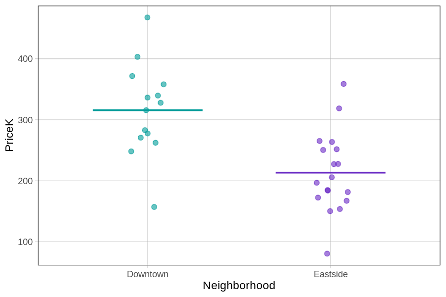
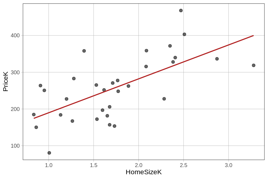
Let’s take a look at a new data set of 32 homes stored in a data frame called Smallville. Similar to the Ames data set, Smallville also has variables such as PriceK, Neighborhood, and HomeSizeK, but for a different town. We have explored two models in Smallville – the Neighborhood model and the HomeSizeK model:

PriceK = Neighborhood + Other Stuff

PriceK = HomeSizeK + Other Stuff

We have visualized these two models in the plots below.

gf_jitter(PriceK ~ Neighborhood, data = Smallville) %>% gf_model(Neighborhood_model)	gf_jitter(PriceK ~ HomeSizeK, data = Smallville) %>% gf_model(HomeSizeK_model)

Notice that these homes from Smallville are from two neighborhoods: Downtown and Eastside. The homes also vary in size – some are smaller than 1000 square feet (or 1K) and others are as big as 3000 square feet.

Both single-predictor models appear to explain some of the variation in home prices; knowing what neighborhood a home is in helps us to make a better prediction of its price, as does knowing its size. Neither model, however, explains all the variation in home prices. There is still plenty of unexplained error (Other Stuff).

We could just choose the single-predictor model that works best. Write some code to make the ANOVA tables from these two models (we have already saved them as the Neighborhood_model and the HomeSizeK_model) to see which one explains the most variation in PriceK.

Analysis of Variance Table (Type III SS)
 Model: PriceK ~ Neighborhood

                                 SS df        MS      F    PRE     p
 ----- --------------- | ---------- -- --------- ------ ------ -----
 Model (error reduced) |  82399.351  1 82399.351 16.842 0.3595 .0003
 Error (from model)    | 146778.142 30  4892.605                    
 ----- --------------- | ---------- -- --------- ------ ------ -----
 Total (empty model)   | 229177.493 31  7392.822  
       

Analysis of Variance Table (Type III SS)
 Model: PriceK ~ HomeSizeK

                                 SS df        MS      F    PRE     p
 ----- --------------- | ---------- -- --------- ------ ------ -----
 Model (error reduced) |  96644.769  1 96644.769 21.876 0.4217 .0001
 Error (from model)    | 132532.724 30  4417.757                    
 ----- --------------- | ---------- -- --------- ------ ------ -----
 Total (empty model)   | 229177.493 31  7392.822    

The better model would be home size. Compared with the empty model, the home size model resulted in a PRE (Proportional Reduction in Error) of 0.42 compared with a PRE of 0.36 for the neighborhood model. More error would be reduced because the predictions from the home size model are more accurate.

But is it possible that we could get an even higher PRE by including both predictors in the model? Another way of asking this question is: could some of the error leftover after fitting the HomeSizeK model be further reduced by adding Neighborhood into the same model? Or, if we knew both the size and neighborhood of a home, could we make a better prediction of its price than if we only knew one or the other?

We could represent this idea like this:

PriceK = HomeSizeK + Neighborhood + Other Stuff