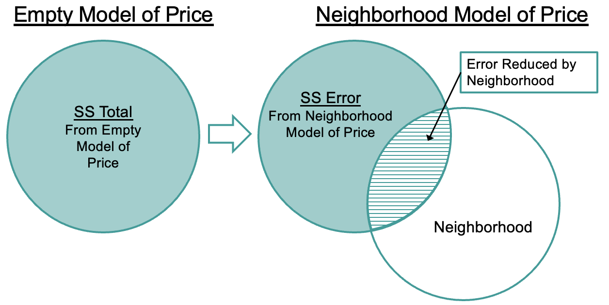
3.5 Error Reduced by the Neighborhood Model
Remember that our goal in adding an explanatory variable to the model was to explain variation in the outcome variable, or to put it another way, reduce error compared with the empty model.
To know that error has been reduced, and by how much it has been reduced, we will compare the sum of squared errors for the empty model with the sum of squared errors from the neighborhood model. If the sum of squared errors from the neighborhood model is smaller, then it has reduced error compared to the empty model.
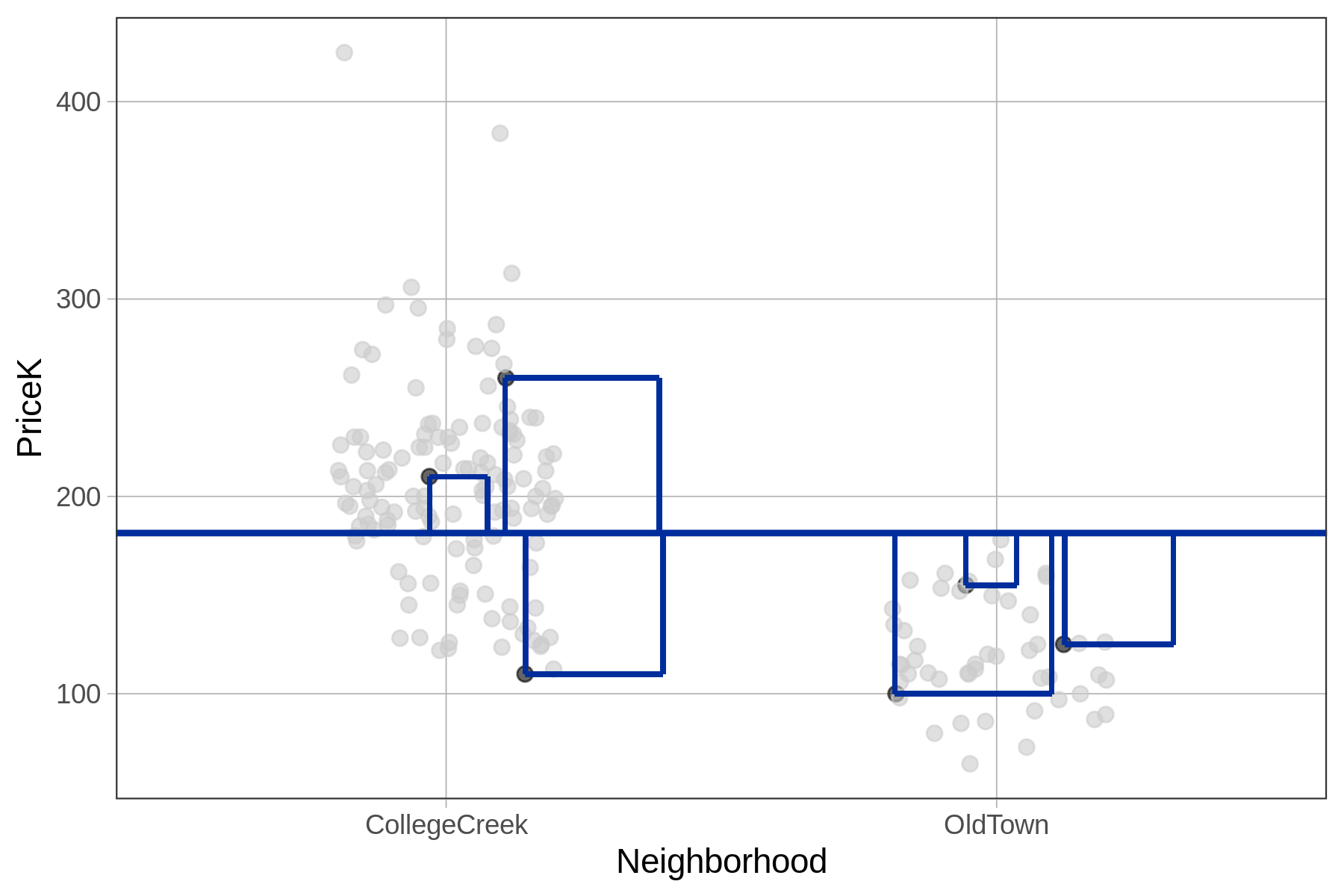
For the empty model, we take each residual from the model prediction (the mean for all homes) and square it. Then we add up these squared residuals to get the total sum of squares. The special name we use to refer to the total squared residuals from the empty model is SST, or Sum of Squares Total.
We have illustrated this idea for our subsample of six data points in the left panel of the figure below. As in the previous figure, the residuals are represented by the vertical lines from each data point to the model prediction. The square of each of these residuals is represented, literally, by a square.
| SS Total, Sum of Squared Residuals from empty model | SS Error, Sum of Squared Residuals from neighborhood model |
|---|---|
|
|
|
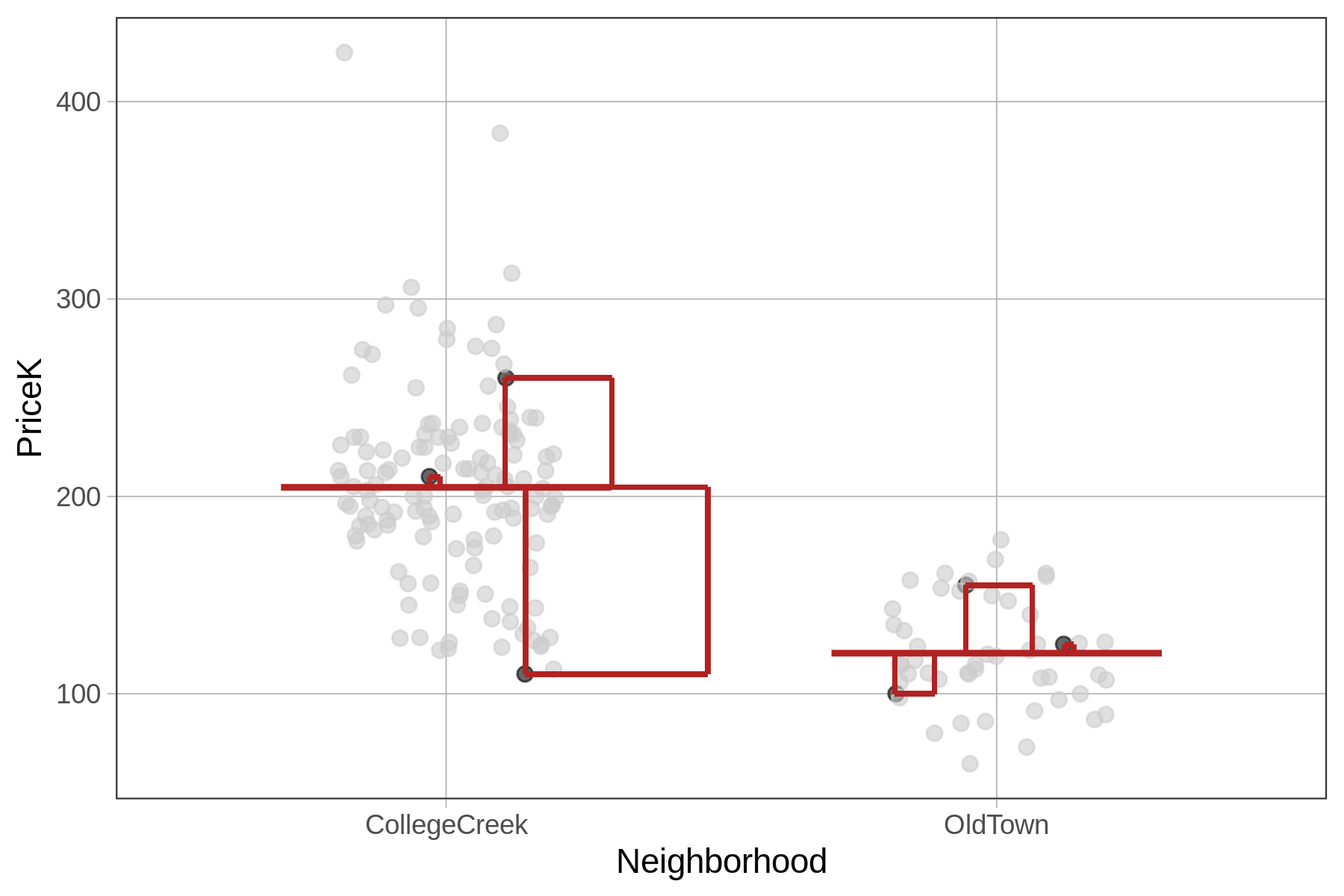
For the neighborhood model (represented in the right panel of the figure above), we take the same approach, only this time the residuals are based on the model predictions of the neighborhood model. Again, we can sum up these squared residuals across the whole data set to get the sum of squared errors from the model.
Although the procedure for calculating sums of squares is identical for the empty and neighborhood models, for the neighborhood model (and indeed, for all models other than the empty model) we call this sum the SSE, or Sum of Squared Errors.
When R fits a model, it minimizes the sum of squared residuals. For the empty model we call this sum of squared errors the SS Total (SST) because it represents the total error in the outcome variable when there are no explanatory variables in the model. For all other models, it is called the SS Error (SSE).
To fit the empty model, R finds the particular value of \(b_0\) that produces the lowest possible SS Total for this data set, which we know is the mean of PriceK. To fit the neighborhood model, R finds the particular values of \(b_0\) and \(b_1\) that produce the lowest possible SS Error for this data set.
Using SS to Compare the Neighborhood Model to the Empty Model
To calculate the sum of squares for each model, we don’t have to add a new column to the data frame. We can, instead, just generate the residuals from each model and save them in an R object, then square them, and then sum them.
In the code window below we have entered code to calculate the SS Total for the empty model. Add some code to calculate SS Error for the Neighborhood model. (We already have created and saved the two models: empty_model and Neighborhood_model.)
require(coursekata)
# This codes saves the best fitting models
empty_model <- lm(PriceK ~ NULL, data=Ames)
Neighborhood_model <- lm(PriceK ~ Neighborhood, data=Ames)

# This code squares and sums the residuals from the empty model
sum(resid(empty_model)^2)

# Write code to square and sum the residuals from the Neighborhood model
sum(resid(Neighborhood_model)^2)
ex() %>% {
  check_function(., "sum", 1) %>%
    check_result() %>% check_equal()
  check_function(., "sum", 2) %>%
    check_result() %>% check_equal()
}633717.215434616372813.203806715We can see from this output that we have, indeed, reduced our error by adding Neighborhood as an explanatory variable into the model. Whereas the sum of squared errors around the empty model (SS Total) was 633,717, for the Neighborhood model (SS Error) it was 372,813. We now have a quantitative basis on which to say that the Neighborhood model is a better model of our data (though perhaps not of the DGP).
This idea is visualized in the figure below.