3.10 Using ANOVA Tables to Compare Models

We have covered a lot in this chapter, getting into the nuts and bolts of statistical models. We have learned how to specify both group and regression models with notation of the GLM, which shows us the largely similar nature of these models. We also have learned how to fit the models, interpret the parameter estimates, and calculate the sum of squared error left after fitting each model.

We already had developed, in a previous chapter, the concept of SS Total from the empty model. Now we can calculate SSE for each complex model, and compare SSE to SST in order to see how much error we have reduced by fitting a more complex model.

Leftover Error from Three Models

The table below summarizes the sums of squares leftover after fitting each of the three models we have been considering. All of these are calculated the same way, by summing the squared residuals from the model predictions.

The more error there is leftover after fitting a model, the less of the total variation is explained. The empty model tells us how much total variation there is in the outcome variable. SS Error tells us how much of that error remains unexplained after fitting a more complex model.

Using supernova() to Print the ANOVA Table

Although we have been building these calculations from the residuals up, we now will show you an easier way to summarize the various sums of squares using ANOVA tables.

We introduced the supernova() function earlier as a way of calculating SST for the empty model. Now let’s return to it and see what it tells us about the more complex models we have been fitting.

We have created and saved two models in the code window below: empty_model and Neighborhood_model. Run the code as is and you will get the ANOVA table for the empty_model. Add another line of supernova() code to get the ANOVA table for the Neighborhood_model.

Analysis of Variance Table (Type III SS)
 Model: PriceK ~ Neighborhood
 
                                 SS  df         MS       F    PRE     p
 ----- --------------- | ---------- --- ---------- ------- ------ -----
 Model (error reduced) | 260904.012   1 260904.012 128.068 0.4117 .0000
 Error (from model)    | 372813.204 183   2037.231                     
 ----- --------------- | ---------- --- ---------- ------- ------ -----
 Total (empty model)   | 633717.215 184   3444.115   

There is a lot going on in this table. For now, let’s just focus on the column labeled SS, which by now you know stands for sum of squares. Notice that supernova() automatically generates the SST (633717) and SSE (372813). We don’t need to run supernova() separately for the empty model and the Neighborhood model; both are readily available in the output.

Partitioning Sums of Squares

We have already discussed the last two numbers in the SS column of the ANOVA table: SSE and SST. But what is the first number (260904)?

Analysis of Variance Table (Type III SS)
 Model: PriceK ~ Neighborhood
 
                                 SS  df         MS       F    PRE     p
 ----- --------------- | ---------- --- ---------- ------- ------ -----
 Model (error reduced) | 260904.012   1 260904.012 128.068 0.4117 .0000
 Error (from model)    | 372813.204 183   2037.231                     
 ----- --------------- | ---------- --- ---------- ------- ------ -----
 Total (empty model)   | 633717.215 184   3444.115   
 

This new type of sum of squares is called the SS Model. SS Model (or SSM) represents the amount of error (measured in sums of squares) that has been reduced by the complex model (in this case the neighborhood model) in comparison with the empty model.

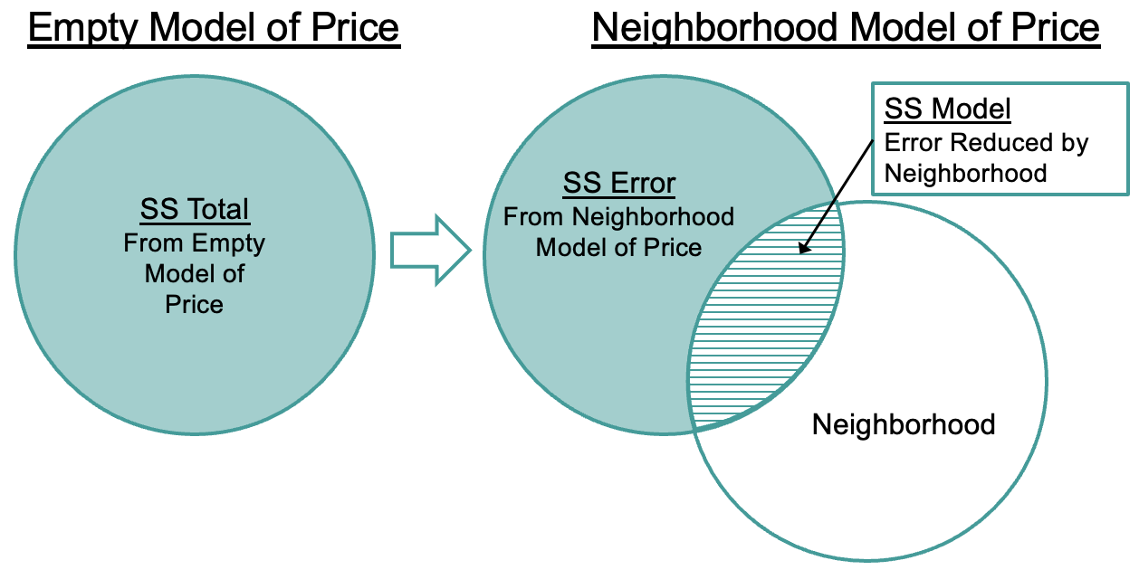
These three different sums of squares in the ANOVA table (SS Model, SS Error, SS Total) reflect a broader idea that we keep bringing up: DATA = MODEL + ERROR. In the case of sums of squares, SS Total literally can be separated into two parts: the error explained by the model (SS Model) and error left unexplained (SS Error). These two parts, added together, equal SS Total.

You can use a calculator (or R) to verify that the numbers in the ANOVA table for SSM and SSE add up to SST. You already know how to directly calculate SST and SSE using residuals. Now you know one way to calculate SSM, using subtraction: SST - SSE.

You can also see this relationship in the Venn diagrams below where the SST can be separated into two parts: SSE and SSM.