8.2 Sums of Squares for Targeted Model Comparisons
Having represented the partitioning of sums of squares in the Venn diagram, let’s connect those parts to all the sums of squares that appear in the ANOVA table.
supernova(lm(PriceK~ Neighborhood + HomeSizeK, data = Smallville))Analysis of Variance Table (Type III SS)
Model: PriceK ~ Neighborhood + HomeSizeK
SS df MS F PRE p
------------ --------------- | ---------- -- --------- ------ ------ -----
Model (error reduced) | 124403.028 2 62201.514 17.216 0.5428 .0000
Neighborhood | 27758.259 1 27758.259 7.683 0.2094 .0096
HomeSizeK | 42003.677 1 42003.677 11.626 0.2862 .0019
Error (from model) | 104774.465 29 3612.913
------------ --------------- | ---------- -- --------- ------ ------ -----
Total (empty model) | 229177.493 31 7392.822
We have already discussed the rows labeled Model, Error, and Total. Let’s turn our attention to the rows labeled Neighborhood and HomeSizeK, one row for each of the two predictor variables. The SS on the Neighborhood row represents the effect of neighborhood after controlling for home size while the SS on the HomeSizeK row represents the effect of home size after controlling for the neighborhood.
Now that we know that regions A and C are in the ANOVA table, we might wonder: where is the B? B, which represents the part of PriceK related to both neighborhood and home size, is not explicitly in the ANOVA table but we can see it in there with a little mental work.
The SS Model represents A+B+C but the two rows with the variable names (Neighborhood and HomeSizeK) only show us A and C.
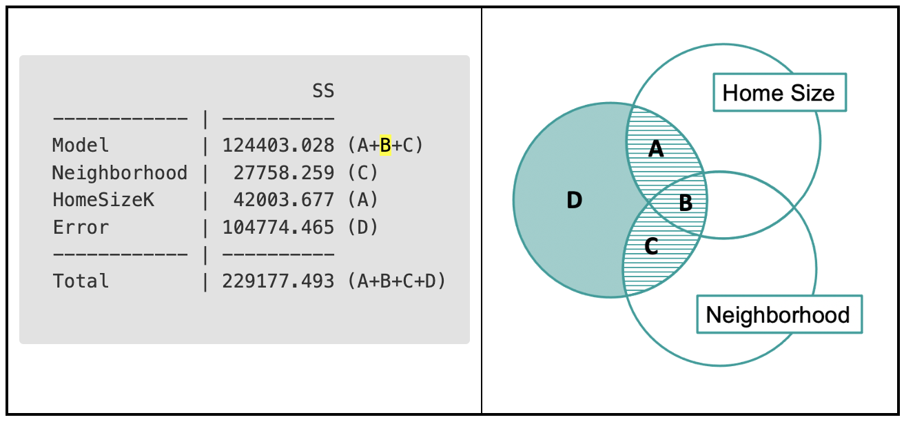
B is the difference between the SS for the whole model and the sum of the two rows (A+C). If there is a large overlap between the two variables (if neighborhood and home size are very much related to each other), then that difference is greater. It’s also possible (though it’s not true in this case) that B could be negative. A+B+C (but not A+C) add up to SS Model.
Thinking with Residuals
So far we have represented sums of squares both in Venn diagrams and in the ANOVA table. We also can calculate the sums of squares directly from the residuals that are leftover after making predictions from a model.
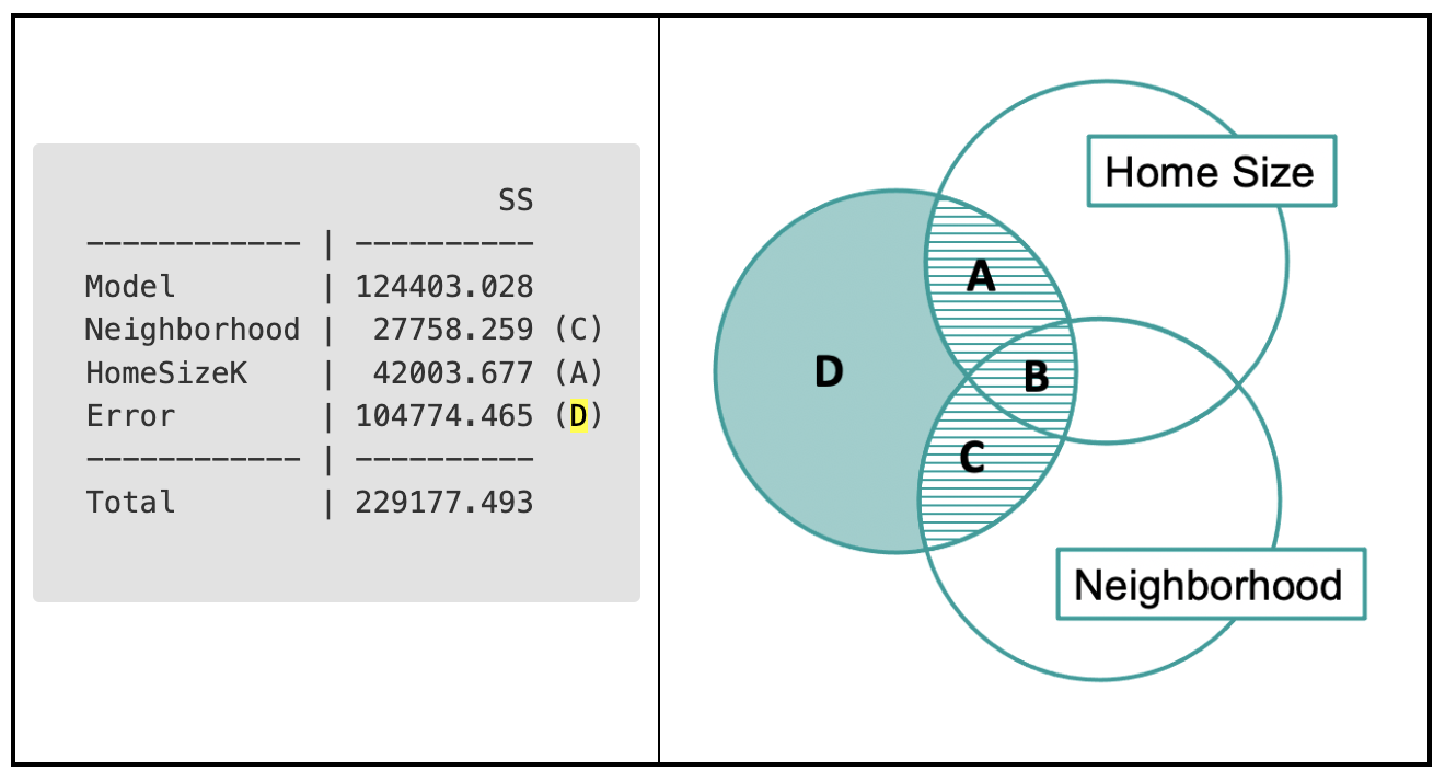
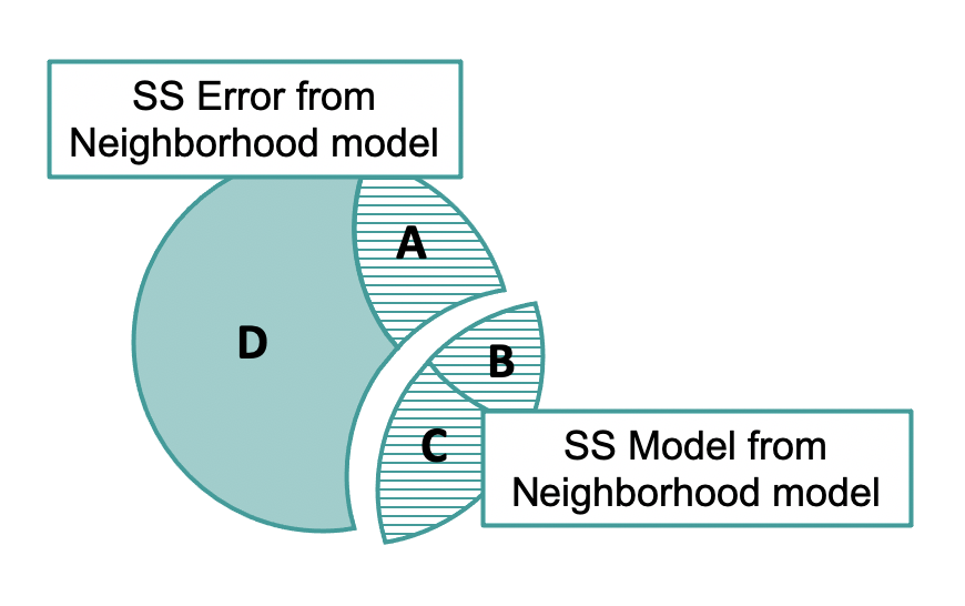
This multivariate ANOVA table is quite powerful. We can also find in it the SS Error from the single-predictor Neighborhood model with a little bit of mental work.
The sum of squares leftover after fitting the single-predictor neighborhood model is not directly available in the multivariate ANOVA table. But, we can calculate it by adding up regions A (which is the SS for HomeSizeK, or 42,003.677) and D (SS Error for the multivariate model, 104,774.465). If we add these two together, we would get 146778.142.
To find this number another way we can fit the neighborhood model, save the residuals from this model, then square and sum them. See if you can do this in the code window below.
require(coursekata)

# delete when coursekata-r updated
Smallville <- read.csv("https://docs.google.com/spreadsheets/d/e/2PACX-1vTUey0jLO87REoQRRGJeG43iN1lkds_lmcnke1fuvS7BTb62jLucJ4WeIt7RW4mfRpk8n5iYvNmgf5l/pub?gid=1024959265&single=true&output=csv")
Smallville$Neighborhood <- factor(Smallville$Neighborhood)
Smallville$HasFireplace <- factor(Smallville$HasFireplace)
# this fits the Neighborhood model
Neighborhood_model <- lm(PriceK ~ Neighborhood, data=Smallville)

# this saves the residuals
PriceK_N_resid <- resid(Neighborhood_model)

# square and sum the residuals
Neighborhood_model <- lm(PriceK ~ Neighborhood, data=Smallville)
PriceK_N_resid <- resid(Neighborhood_model)
sum(PriceK_N_resid^2)
# temporary SCT
ex() %>% check_error()146778.141887714We got the same number we arrived at by adding regions D and A together from the multivariate model!
Go ahead and get the ANOVA table for the Neighborhood model in the code window below. See where the 146,778 shows up.
require(coursekata)

# delete when coursekata-r updated
Smallville <- read.csv("https://docs.google.com/spreadsheets/d/e/2PACX-1vTUey0jLO87REoQRRGJeG43iN1lkds_lmcnke1fuvS7BTb62jLucJ4WeIt7RW4mfRpk8n5iYvNmgf5l/pub?gid=1024959265&single=true&output=csv")
Smallville$Neighborhood <- factor(Smallville$Neighborhood)
Smallville$HasFireplace <- factor(Smallville$HasFireplace)
# this fits the Neighborhood model
Neighborhood_model <- lm(PriceK ~ Neighborhood, data=Smallville)

# find the ANOVA table
Neighborhood_model <- lm(PriceK ~ Neighborhood, data=Smallville)
supernova(Neighborhood_model)
# temporary SCT
ex() %>% check_error()Analysis of Variance Table (Type III SS)
Model: PriceK ~ Neighborhood
SS df MS F PRE p
----- --------------- | ---------- -- --------- ------ ------ -----
Model (error reduced) | 82399.351 1 82399.351 16.842 0.3595 .0003
Error (from model) | 146778.142 30 4892.605
----- --------------- | ---------- -- --------- ------ ------ -----
Total (empty model) | 229177.493 31 7392.822