2.6 Fitting the Empty Model
The first step in modeling data is to decide what model you want to create – e.g., the empty model. This decision is often referred to as specifying the model. The next step is to fit the model to the data.
In the case of the empty model, fitting the model means simply calculating the mean of the outcome variable for all observations in the data set. It may seem like we are making a big deal out of nothing by calling this “fitting the model.” But it’s important, because as models get more complex later, fitting the model won’t be as simple as calculating the mean.
Introducing the lm() Function
In R there are many ways to calculate the mean of a variable. We could use favstats(), for example. But we are going to teach you another function for fitting the empty model that can later be used to fit much more complex models. This function is lm(), which stands for “linear model.” Here’s the code we use to fit the empty model of PriceK, followed by the output.
lm(PriceK ~ NULL, data = Ames)Call:
lm(formula = PriceK ~ NULL, data = Ames)
Coefficients:
(Intercept)
181.4Although the output of lm() might seem a little strange, with words like “Coefficients” and “Intercept,” it does give you back a single number, which is the predicted value of PriceK under the empty model.
In the code window below, we’ve written a line of code to calculate the favstats() for PriceK. Add in the code to fit the empty model of PriceK using lm(). Compare the results of the two functions.
require(coursekata)
# here's code to find empty model using favstats()
favstats(~ PriceK, data = Ames)

# write code to find the empty model using lm()
# here's code to find empty model using favstats()
favstats(~ PriceK, data = Ames)

# write code to find the empty model using lm()
lm(PriceK ~ NULL, data = Ames)
ex() %>% {
  check_function(., "favstats") %>% check_result() %>% check_equal()
  check_function(., "lm") %>% check_result() %>% check_equal()
}The result of fitting the empty model using lm() is the same as calculating the mean of the distribution of PriceK: 181.4.
We sometimes refer to the results of the lm() function as the model fit. It will be helpful to save this model fit in an R object so we can use it later. Here’s code that uses lm() to fit the empty model, then saves the results in an R object called empty_model:
empty_model <- lm(PriceK ~ NULL, data = Ames)If you want to see what the model estimates are after running this code, you can just type the name of the object where you saved the model. Try it in the code block below.
require(coursekata)
# this saves the empty model of PriceK
empty_model <- lm(PriceK ~ NULL, data = Ames)

# write code to print the contents of empty_model
# this saves the empty model of PriceK
empty_model <- lm(PriceK ~ NULL, data = Ames)

# write code to print the contents of empty_model
empty_model
ex() %>% check_output_expr('empty_model')Comparing Models
As we have said before, all models are wrong, but some are less wrong than others. The reason we gave for introducing the empty model was that it provides a simple model to which we can compare a more complex one.
Let’s go back, briefly, to discuss what we have learned so far in relation to the comparison of these two models:
PriceK = Neighborhood + Other Stuff PriceK = Mean + Other Stuff
Which of these models is a better representation of the Ames data? So far we have only quantified the empty model; in the next chapter we will quantify the neighborhood model. But even just quantifying the empty model can help us think about the process of comparing these two models.
Let’s go back and create a jitter plot that shows PriceK as a function of Neighborhood. We’ve put the code in the window below. (You can run it if you want, just to remember what it does.)
We’ll teach you a new function called gf_model() which overlays the model predictions on top of a graph. gf_model() takes a model as its input (the part in the parentheses). If we save the empty model in an R object, we can put it right into the function like this: gf_model(empty_model).
Try chaining gf_model(empty_model) onto the jitter plot in the code window below.
require(coursekata)
# this saves the empty model
empty_model <- lm(PriceK ~ NULL, data = Ames)

gf_jitter(PriceK ~ Neighborhood, data = Ames, width = .1)
# this saves the empty model
empty_model <- lm(PriceK ~ NULL, data = Ames)

gf_jitter(PriceK ~ Neighborhood, data = Ames, width = .1) %>%
  gf_model(empty_model)
ex() %>% check_function("gf_model") %>% {
  check_arg(., "model") %>% check_equal()
  check_result(.) %>% check_equal()
}
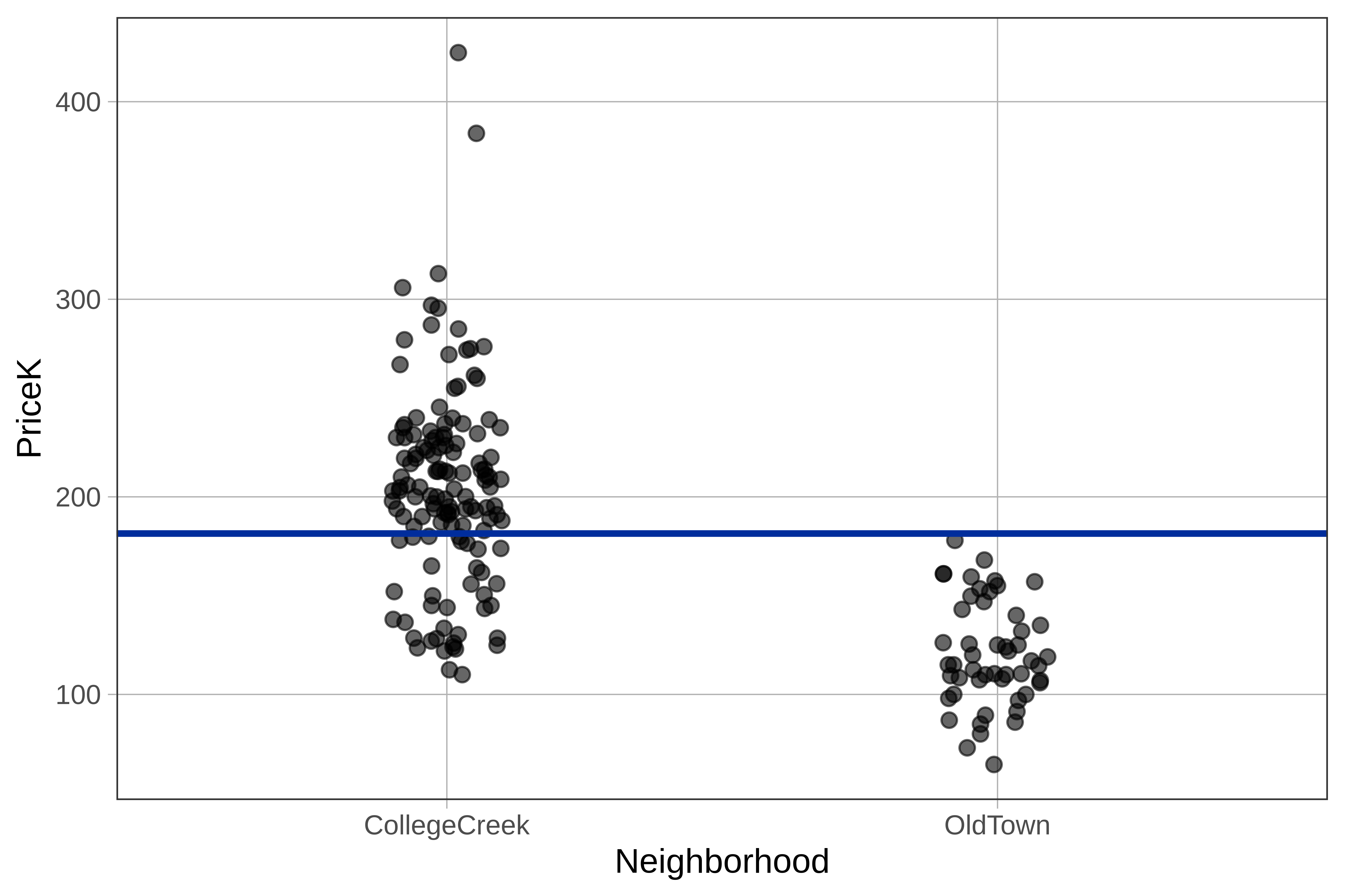
We haven’t yet represented predictions of the neighborhood model on this jitter plot, but we can see the predictions of the empty model represented as a horizontal line. If we use the empty model, we would predict the price of the next home sale to be $181.4K, regardless of what neighborhood the home is in. This is why the horizontal line goes all the way across the two categories College Creek and Old Town – no matter which neighborhood, this model predicts the same value.
By overlaying the prediction on the jitter plot, it helps us see the limitations of the empty model. In particular, we can see that if we did know what neighborhood the sale was in, we might want to adjust our prediction of the sales price.