3.12 Comparing Models with PRE

Proportion Reduction in Error (PRE)

One disadvantage of using sums of squares to compare models is that they only make sense when comparing models that use the same outcome variable (e.g., PriceK) and the same data set (e.g., Ames). Just having a larger sample size in your data set will increase your sums of squares. That doesn’t mean, though, that your model is getting better or worse.

A more general way to characterize how good a model fits is by the proportion of the total variation (SS Total) that is explained, or reduced, by the complex model (SS Model). This metric is called the Proportion Reduction in Error, or PRE. You will find it in the supernova table.

Analysis of Variance Table (Type III SS)
Model: PriceK ~ Neighborhood
 
                                 SS  df         MS       F    PRE     p
 ----- --------------- | ---------- --- ---------- ------- ------ -----
 Model (error reduced) | 260904.012   1 260904.012 128.068 0.4117 .0000
 Error (from model)    | 372813.204 183   2037.231                     
 ----- --------------- | ---------- --- ---------- ------- ------ -----
 Total (empty model)   | 633717.215 184   3444.115                    

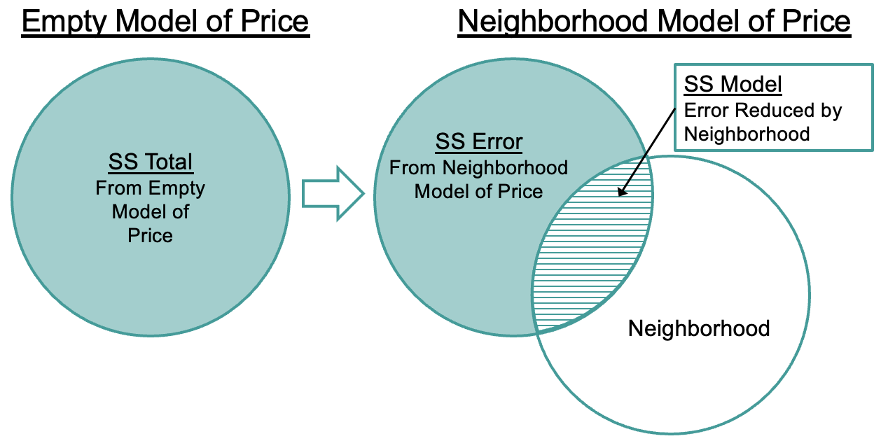
PRE is literally the proportion of error that is reduced by the complex model over the empty model. The total error to be explained is represented by SST. This can be thought of as 100% of the error in PriceK that potentially could be explained.

If we take the part of that total error that can be explained (or reduced) by Neighborhood (SSM) and then divide it by the total error in the outcome variable (SST) we will get PRE.

Total variation in PriceK is represented by the blue circle in the figure below, the part explained by Neighborhood is the overlap between the two circles (striped area). If we take SS Model (the striped area) and divide by SS Total (the whole blue circle), we get PRE.

We can summarize the calculation of PRE with this formula:

\[P\!R\!E = \frac{S\!S_{Model}}{S\!S_{Total}}\]

A PRE of .41 tells us that a lot of the variation in price is explained by the neighborhood model. (In many fields of research, it’s exciting to get a PRE as high as .05.)